History of artificial intelligence · Part 1

Artificial intelligence did not appear suddenly in a single moment or with one great invention. It grew out of questions that people had been working on for centuries — some long before electronic computers even existed. This first part traces the threads that eventually came together to make AI possible, so you can see why each idea was needed and how they connect.

• Probability and learning from evidence. Before any machine could “learn,” statisticians had already worked out how to update a belief when new data arrives, and how to describe relationships between variables. These tools became the mathematical engine of later learning systems.
• Computation, Turing and early neurons. Mathematicians needed a precise definition of what it even means for something to be “computable,” and biologists provided inspiration: if real brains are made of simple cells that combine signals, perhaps machines could imitate them with simple artificial units.
• The birth of AI and early learning systems. In the 1950s researchers finally had both the ideas (statistics + computation) and enough hardware to name their field, build demonstration programs, and make a machine learn from examples for the first time.

As you read through this part, keep asking one guiding question: “What problem was each person trying to solve?” The history makes much more sense when you see every idea as an answer — however partial — to a real difficulty its author faced. You do not need any previous AI or statistics background for what follows; each concept is introduced from scratch.

Before we travel into the past, it helps to agree on what artificial intelligence (AI) means today. AI is a broad field concerned with building engineered systems that carry out tasks we usually associate with intelligent behavior: reasoning through a problem step by step, perceiving the world through sensors such as cameras and microphones, planning a sequence of actions to reach a goal, communicating in language, recognizing patterns, and making decisions under uncertainty. Notice how wide this definition is — it covers everything from a chess program that plans ahead, to a speech assistant that understands your voice, to a robot that avoids obstacles.

Within that broad field sits machine learning (ML), which you can think of as one specific strategy for building intelligence. Instead of having a human hand-write every rule the system should follow, machine learning uses a training procedure: we show the system examples and let an algorithm adjust its internal parameters — numbers that control its behavior — so that it performs better on those examples. The key point is that the program changes itself based on data or experience rather than being given every answer in advance.

However, machine learning does not remove the need for human judgment and careful design. Before you can train anything, someone must still: (1) define a clear task — what exactly should the system do? (2) choose an objective — how will we measure whether it did well or badly? and (3) set up an evaluation — separate data used to check that learning actually worked on cases the machine never saw. These three ingredients frame every learning problem, then and now.

There is one more subtle but important idea in this section: a model that has been trained does not automatically keep improving while you use it. Once training stops, the system typically keeps making predictions with its fixed parameters. If you want it to learn again — for example because new data arrived or the world changed — you must run another update process (that is, retrain). This distinction between “using” a model and “learning/updating” it will reappear throughout the course.

The whole history of AI is usually told as a sequence of ten broad eras. It is worth reading this list once now so you have a mental map, even though most of it will be explained in detail later. The eras are:

1. Statistical foundations (1763–1936): probability and regression tools developed before computers.
2. Computation theory & Turing (1936–1950): precise definitions of what computation is, plus early chess algorithms and Turing’s famous question about machine thinking.
3. Cybernetics & neurons (1943–49): feedback control systems and the first mathematical model of a neuron.
4. The birth of AI (1950s): researchers name their field, build reasoning programs and early learning machines.
5. The first “AI winter” (~1974–80): funding drops when ambitious promises meet hard technical limits.
6. Expert systems (1980s): rule-based programs that encode human knowledge for specific tasks.
7. A second AI winter & renewed connectionism (late 1980s–90s): another funding cycle ends, while neural-network research quietly resumes.
8. Deep learning (2012 onward): large multi-layer networks trained on massive data transform the field.
9. Generative systems (recent years): models that create new text, images and audio.

The most important thing to understand about this timeline is that it is a simplification. Real history does not move in clean stages where one idea switches off exactly when another switches on. Symbolic approaches (reasoning with explicit rules) and learning-based approaches (adjusting parameters from data) developed side by side for decades, often borrowing ideas from each other. Different research communities changed direction at different times in different countries.

So use this list as a handy navigation aid to place people, papers and programs — not as an authoritative claim that every era ended on the date printed next to it. History is continuous; our chapter boundaries are just convenient signposts for learning.

The first chapter goes all the way back to mathematics developed in the eighteenth and nineteenth centuries — a time long before electronic computers existed. This might seem strange at first, but there is one central idea you should take from it: our observations are always incomplete evidence. We almost never see the full truth directly; we only glimpse parts of it through measurements, samples or signals.

A statistical model is precisely a set of assumptions that connects these incomplete observations with something unknown that we actually care about. For example: you observe the heights of parents and their grown children (observations) and want to describe how tall children tend to be given their parents’ height (the relationship between variables). Or you observe some symptoms in a patient and want to know the probability they have a certain disease — but your data only tells you something about the reverse direction, so you need Bayes’ theorem to flip it around.

Three families of statistical tools introduced here became permanent, reusable components inside modern machine-learning systems:

• Bayes’ theorem — how to update a belief when new evidence arrives;
• Regression (linear and logistic) — how to describe relationships between variables and predict categorical outcomes;
• Markov chains — how to model sequences of events where what happens next depends on the current state.

The reason these matter for AI is not merely historical nostalgia. When you later study classification, prediction and sequence models in machine learning, you will be using modern descendants of exactly these ideas. Understanding their origin gives you intuition about why they are built the way they are — and why even very old mathematics can still power state-of-the-art systems.

This section gives you a quick map of the statistical toolkit that would later feed into AI. Each tool solves a different kind of problem, and together they cover most situations you will meet:

• Bayesian inference is about updating uncertainty. You start with some degree of belief (the “prior”), observe evidence, and compute how that evidence should change your belief (giving a “posterior”). It answers: given what I just saw, how confident should I now be?
• Regression is about describing relationships among variables. You have several measured quantities and want to know how one of them tends to vary as the others change — for instance, how a student’s exam score relates to hours studied.
• Markov models are about simplifying sequences. Real events arrive in order (weather day after day, letters in a sentence), and the future often depends on the past. Markov made this manageable with a simplifying assumption: for prediction purposes, everything relevant from the past can be summarized by the current state.
• Logistic and probit models are about predicting categories. Sometimes you do not want to predict a number but which of two outcomes will occur (pass/fail, spam/not-spam). These models take several predictor variables and turn them into a probability between 0 and 1 using different mathematical “link functions.”

Two broader lessons come out of this chapter. First, these scientific tools were developed to answer real questions — about heredity, growth, disease, games of chance — and they became the foundations on which learning systems are built. Second, their continued use today makes an important point: progress in AI does not mean old techniques become useless. Modern machine learning often combines very recent algorithms with these older statistical building blocks. Learning where each one comes from helps you understand what it is good at and when to reach for it.

Bayes’ theorem, named after the Reverend Thomas Bayes, is one of the most important single formulas in statistics and machine learning. It tells you how to answer this everyday question: “How should new evidence change what I believe?” Before seeing any data you have a prior belief; afterwards your updated belief is called the posterior.

The theorem connects three quantities:

• the prior — how likely you thought something was before looking at the evidence;
• the likelihood — how probable the observed evidence would be if your hypothesis were true (and, implicitly, under alternative hypotheses);
• the posterior — how confident you should now be after combining prior and evidence.

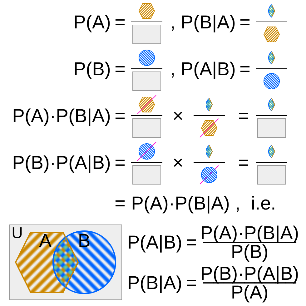
A famous intuition is a medical test. A test might tell us “if the patient has disease D, there is a high probability the result comes back positive” — that is information in one conditional direction (disease → test). But what we actually want to know runs the other way: “given that this patient tested positive, how likely are they really to have D?” Bayes’ theorem lets us reverse the condition using our knowledge of the disease rate and the false-positive chance. This reversal-of-condition is exactly the situation where Bayes shines.

The diagram in this section pictures that relationship between prior, likelihood and posterior visually — worth studying because it fixes the intuition far better than algebra alone.

Two cautions keep the theorem honest. First, mathematically it is an identity: a guaranteed true relationship among probabilities. The work comes from choosing sensible values for its ingredients (the prior and likelihood), which must be specified or estimated by you — the formula does not provide them. Second, later classification methods use Bayes’ idea to compare how likely each class is given an observed data point: instead of asking “is this symptom consistent with disease?”, they compute a probability for each candidate answer and pick the most probable one. That modern technique is the direct descendant of this 1763 formula.

The core idea of linear regression is delightfully simple: to predict one quantity (the response) from others (the predictors), you assume the response can be written as a weighted sum of the predictors, plus some constant. For instance, with two predictors the model looks like:

where x are the inputs (e.g., hours studied and previous grades), w are weights telling you how strongly each input matters, b is a baseline constant, and y is your predicted output (the exam score). The weights are the numbers we want to discover from data.

The classic way to fit such a line — called the method of least squares, published by Legendre in 1805 and given a deeper probabilistic treatment by Gauss in 1809 — is to choose the weights that make the predictions as close as possible to the true values, measured by minimizing the sum of the squared differences (the “residuals”) between prediction and reality. Squaring makes large errors count disproportionately, which pushes the solution toward being consistently good rather than wildly wrong on a few points.

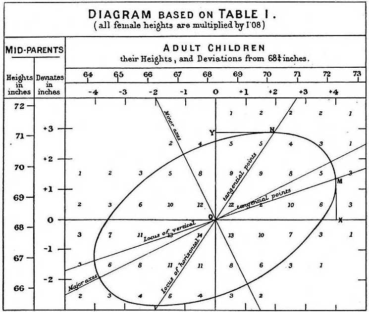
The word regression itself comes from an odd place: Sir Francis Galton’s 1886 study of heights across generations. He noticed that very tall parents tend to have children who are somewhat shorter, and short parents tend to have children somewhat taller — as if offspring were being pulled back toward the average height of the whole population. Galton called this pull “regression toward mediocrity.” The name stuck even though today we use regression for far more general problems than heredity.

Two warnings keep your understanding accurate. First, choosing a linear model is not a claim that reality is always linear; it is a choice of representation — one that happens to be simple, fast and easy to inspect (you can literally read the weights to see what matters). Sometimes that simplicity is worth more than perfect accuracy. Second, finding an association between variables does not prove causation: if tall parents have tall children, we cannot conclude that being tall “causes” height in children — genes and environment explain both. Linear regression describes relationships; establishing what would happen if you intervened (change X to make Y change) is a different, harder problem.

The Galton figure above shows his original plot of parent–child heights, where the elliptical cloud of points reveals how the two are related — an early ancestor of today’s scatter plots and trend lines.

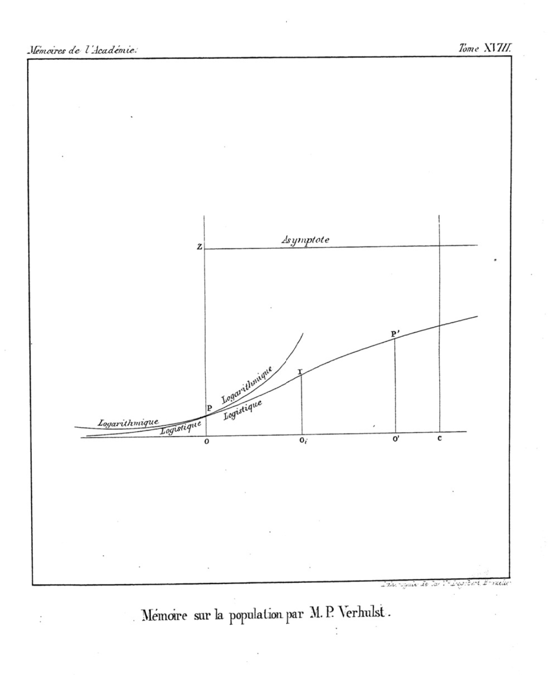
The story of logistic regression starts, surprisingly, with biology rather than AI. In the early nineteenth century mathematicians studied how populations grow over time — plants, animals or bacteria in a limited environment. A population cannot keep growing forever at exponential speed: food and space run out. The mathematician Pierre-François Verhulst proposed in 1838 an S-shaped (sigmoid) growth curve that rises quickly in the middle but flattens toward an upper limit — you can see exactly these curves in his figure below.

The key historical point is to keep two things separate:

1. The logistic curve for population growth (Verhulst, 1838) — a descriptive model of how a quantity grows over time toward a cap.
2. Modern logistic regression (popularized by Berkson in 1944) — a statistical tool for predicting categorical outcomes such as pass/fail or yes/no. These are different models that happen to share the same S-shaped mathematical function.

So what does modern logistic regression actually do? Imagine you have several predictors and want to predict one of two categories (for example: will this email be spam?). A natural first attempt is a linear score — add up weighted inputs just like in linear regression. But that gives an unbounded number, whereas probabilities must always lie between 0 and 1. Logistic regression solves the mismatch by passing the linear score through the sigmoid curve: any real-number score gets compressed into a value strictly between 0 and 1, which we interpret as a probability.

This is why the two ideas are fully compatible rather than contradictory: the coefficients still act in a clean, linear way inside the score (easy to interpret — larger weight means more influence), while the sigmoid makes sure the final output behaves like a probability. This combination of an easily interpreted linear core and a bounded probabilistic output is exactly what made logistic regression so popular for classification.

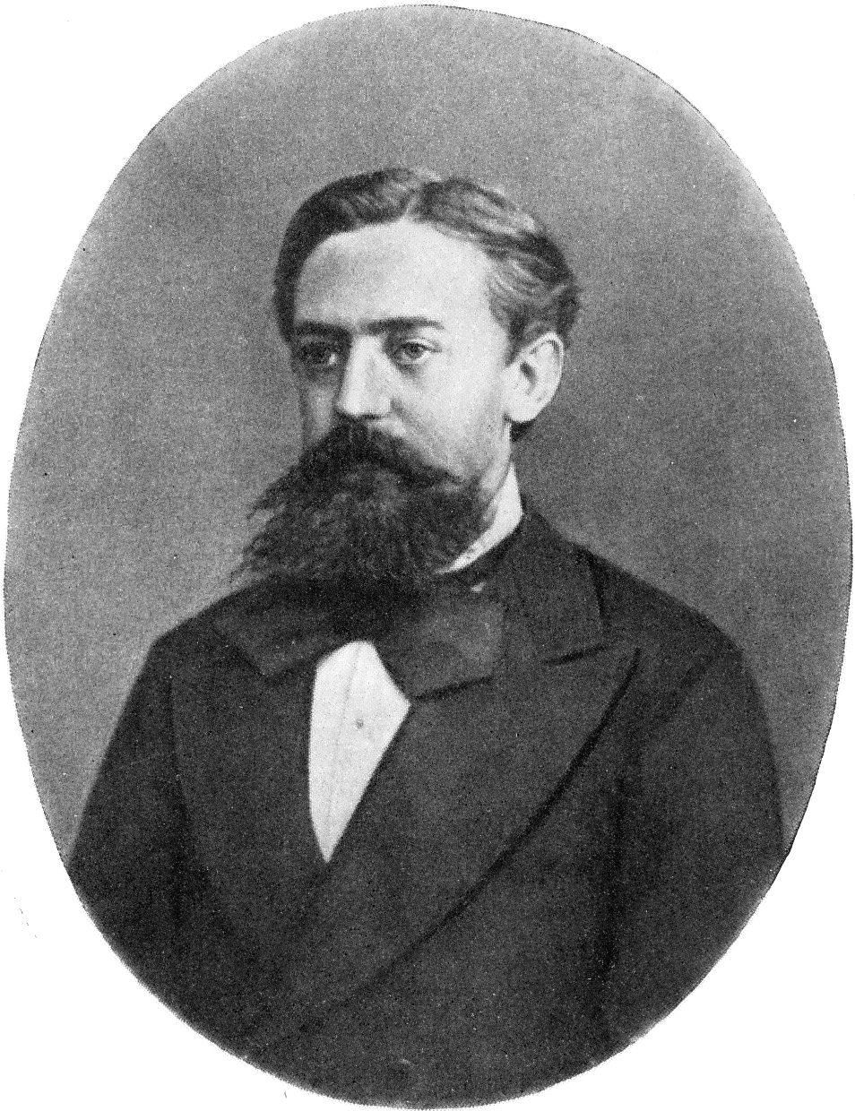
A Markov chain, introduced by the Russian mathematician Andrey Markov, is a tool for modeling things that happen one after another in time — weather each day, letters in a text, positions of a moving robot. The central idea is the Markov property: when predicting what comes next, everything you need to know from the entire past can be summarized by where you are right now (the current state). Formally: given the present state, the next state does not depend on any earlier history.

It is crucial to understand what this does and does not say. It does not claim the past was irrelevant — after all, your current state may already encode a great deal of history (today’s rainy sky tells you something about yesterday’s weather). What it claims is that for prediction purposes you can safely discard everything except the present state; nothing further back adds new predictive information. This simplification is what makes sequential modeling tractable: instead of needing to remember every detail since the beginning of time, you only track one current state.

Why does this matter so much for AI? Because enormous numbers of problems are inherently sequential:

• predicting tomorrow’s weather from today’s;
• autocomplete and language models, where each next word depends on the context built up so far;
• tracking a moving object when you only get noisy measurements.

The last example leads to an especially powerful extension called hidden Markov models. There we assume there is an underlying state (e.g., the true position of a robot or the actual weather) that we cannot observe directly; instead, at each step we receive only indirect evidence about it. This idea — inferring a hidden cause from observable effects over time — appears in speech recognition and many other sequence-based machine-learning systems you will meet later.

The probit model is a close cousin of logistic regression, and the two are so similar that they are often taught together. Both solve the same fundamental problem: how to turn predictor variables into a probability (between 0 and 1) for one of two outcomes. The only real difference between them is which mathematical function — which link function — does the turning.

• Logit uses the logistic sigmoid curve we met in the previous section.
• Probit instead uses the standard normal (bell-curve) cumulative distribution function from statistics.

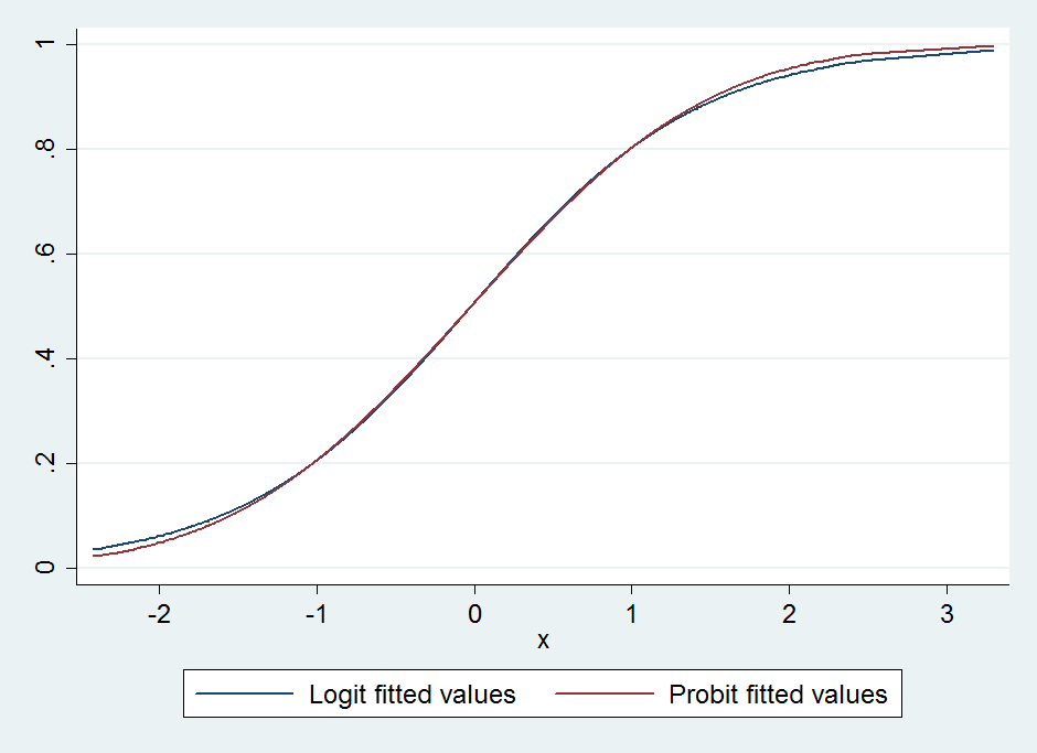
where Φ is the normal “S-curve.” Both are S-shaped, both map any score to a value between 0 and 1, and their graphs look almost identical across most of the input range — you can see this side by side in the figure above. They only differ noticeably out near the tails (the extreme low and high ends), where one curve approaches its limits slightly faster than the other.

What should a student take away from such similar models? The point is not “memorize which is better” but to notice how related statistical formulations can coexist for decades. Neither model is intrinsically correct; each embodies slightly different assumptions about the underlying probability distribution, and researchers pick between them based on those assumptions and on their analytical context (some fields conventionally use one or the other).

And here is an important historical lesson: just because logistic regression became far more popular does not mean probit has become extinct. Popularity in research fashions says little about a method’s validity — it remains perfectly useful when its assumptions fit. This healthy skepticism toward “the winner takes all” view of methods is exactly the attitude you should carry into the rest of this course.

The second chapter shifts focus from statistics to the very nature of computation itself. Its central questions are deceptively simple but enormously deep:

• What makes a procedure computable? Is there a precise boundary between problems that can be solved by following an algorithm and those that cannot, no matter how clever or fast our machine is?
• How should we evaluate whether a machine behaves intelligently? What evidence would convince us it “thinks,” when the machine’s inner workings differ so much from ours?

A striking feature of this era is that many of these ideas were worked out in theory and on paper — with formal models, diagrams and hand-simulated examples — years before any computer hardware could actually run them comfortably. The thinkers involved (above all Alan Turing) did not wait for machines to exist; they first created precise conceptual tools to describe what a machine could do in principle.

In this chapter you will meet the abstract “Turing machine” that defines computation itself, an early chess-playing procedure whose games were simulated by hand because no computer was available, and Turing’s famous reframing of the question “can machines think?” into a practical test based on observable behavior. Together these set up both the theoretical foundations and the philosophical ambitions that AI would build on.

This section asks you to separate three questions that are easy to confuse but actually quite distinct. Keeping them apart is essential for understanding everything that follows:

1. Does an effective procedure even exist? This is the question of computability, studied by Alonzo Church and Alan Turing in the 1930s. Given a problem, is there any algorithm at all — regardless of how long or slow it would run — that always solves it? Some problems simply have no algorithmic solution.
2. How should the procedure choose among many actions? This is the question of search. Once an algorithm exists (as in chess), there are usually huge numbers of possible steps. How does a program decide which move to try, given limited time and memory? Early chess programs explored exactly this.
3. What evidence should be used to judge intelligent behavior? This is the philosophical/evaluation question Turing later addressed: rather than debating internal “consciousness,” how about observing what the machine does in conversation or on a task?

The distinction between computability and speed/practicality deserves special emphasis. A problem can be perfectly computable — an algorithm for it provably exists — yet take so long that no real computer could finish within a human lifetime. Computability tells you whether a solution is possible in principle; speed concerns how to make the solution usable in practice, which often requires clever shortcuts and heuristics rather than brute force.

So as you move through this chapter, keep asking which of these three questions each contribution answers: whether an effective procedure exists (Church–Turing), how it chooses actions under constraints (chess search), or what evidence counts for intelligent behavior (the imitation game).

In the mid-1930s mathematicians were wrestling with a deceptively tricky question: what does it precisely mean to say that some procedure is “effectively calculable”? Humans had computed things for millennia, but nobody could define sharply where computation ends and impossibility begins. Two researchers independently produced formal answers in the same period:

• Alonzo Church invented the lambda calculus, a symbolic system for expressing computations as functions applied to arguments (this is the direct ancestor of functional programming languages).
• Alan Turing defined an idealized device — now called the Turing machine — consisting only of an infinitely long tape divided into cells, a read/write head, and a small table of rules telling it how to move and change symbols.

Astonishingly, Church’s lambda calculus and Turing’s machines turned out to describe exactly the same class of computable functions: anything one can compute with one formalism, you can compute with the other. The Church–Turing thesis is the claim that this shared formal notion captures precisely what we mean by “effectively calculable” in ordinary informal language — in other words, that these abstract devices define the true limits of any possible computation.

The wooden-machine video below shows a modern physical implementation built to demonstrate Turing’s idea with real moving parts. Please note it is not a historical recording from 1936; it is a recent educational demonstration of an old concept, which makes the abstract model tangible and easier to grasp.

A crucial distinction: the Church–Turing thesis says that formal computability matches informal calculability — but it does not say every interesting problem has a solution. On the contrary, this line of work produced one of the most important negative results in all of mathematics. Turing and others studied the “decision problem” (whether some logical statement is valid) and proved that such problems can be genuinely undecidable: there exist well-posed questions for which no algorithm can always give an answer, ever — not just a slow one. The undecidability result is a hard mathematical theorem; equating informal “effective calculation” with formal computability is the thesis (a widely accepted but philosophical identification). Understanding that some problems are provably unsolvable-by-algorithm gives AI its honest boundaries: no amount of cleverness or computing power can overcome certain fundamental limits.

Chess has fascinated AI researchers from the very beginning — and TuroChamp, devised by Alan Turing together with David Champernowne in the late 1940s, is one of the earliest attempts to express how a person plays chess as a step-by-step algorithm.

To understand its significance you must appreciate two things about chess that make it hard for computers: (1) the rules are crisp and unambiguous, which is good — but (2) the number of possible games is astronomically large. From any position there can be dozens of legal moves; after each move your opponent replies with one of theirs; after only a few turns the branching choices multiply into millions or more of possibilities. No machine could ever examine them all, and no human plays that way either.

So TuroChamp’s approach was guided search. The program would look ahead over several moves (searching through promising continuations rather than every possible one), evaluate how good each resulting position looked using a scoring function — counting material like pieces, plus positional factors such as mobility and development — and then choose the move that led to the best-scored outcome. This combination of search + evaluation became the template for computer chess (and many other games) for decades.

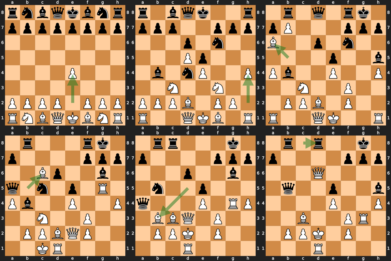
The most instructive historical point is the enormous gap it reveals between specifying a procedure and actually running it on hardware. In 1952 there was no general-purpose computer available to Turing that could execute TuroChamp at playable speed, so the game shown above — TuroChamp (white) versus a friend named Alick Glennie (black), in which White won — was simulated by hand. Turing and Champernowne literally performed each step of the algorithm manually with pencil and paper. For this reason we call it an early chess algorithm, not the first completed computer implementation; the distinction keeps us accurate about what actually existed.

TuroChamp teaches a lasting lesson: you can design a perfectly correct procedure on paper while practical machines cannot yet run it comfortably — exactly the theory-vs-hardware gap highlighted in this chapter. And it shows why chess became AI’s favorite testbed: its strict rules and immense branching space force any program to search intelligently rather than rely on brute-force enumeration, which is precisely the kind of guided reasoning researchers hoped would scale to other “intelligent” tasks.

In his famous 1950 paper Computing Machinery and Intelligence, Alan Turing asked what became the defining question of AI: “Can machines think?” But rather than getting lost in endless philosophical debate over the meaning of “think,” he cleverly proposed a way to make the question testable — he called it the imitation game.

The setup works like this. A human examiner sits in one room and communicates, purely through typed text messages, with two hidden entities: a real person and a machine. The examiner’s job is to figure out which of the two is the machine by asking questions and reading the replies (the kind of exchange familiar from modern chat). The physical identities are completely concealed — no voice, face or body language — so all the evidence available is what each side types back.

Two features make this proposal important for AI:

• It focuses on observable behavior, not internal consciousness. Instead of arguing about whether a machine “really feels” or “truly understands,” we evaluate what it does. If the examiner cannot reliably tell machine from human, then — for behavioral purposes — the machine has passed.
• It sidesteps an impossible definition. Turing deliberately avoided giving an unrestricted definition of thinking. He turned a vague metaphysical question into a concrete, repeatable test based on text interaction alone (today we would recognize this as essentially a chatbot evaluation).

The idea was hugely influential and is still discussed constantly in AI ethics and research — but you should also understand its limitations. The imitation game is not universally necessary or sufficient for every meaning of intelligence: one could imagine intelligent beings that would fail it (e.g., a brilliant non-verbal thinker), and systems that might pass it without anything like genuine understanding. It is best understood as Turing’s pragmatic reframing — a way to make progress on the question by replacing “thinking” with observable conversational competence.

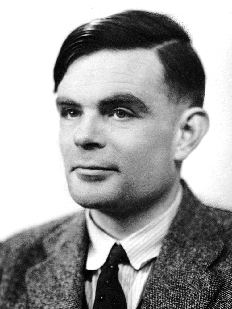
The linked paper, Computing Machinery and Intelligence, not only lays out this framing but also anticipates and answers many objections people raised against machine intelligence in 1950 — an early model of careful, structured reasoning about AI that remains worth reading today. The portrait below shows Turing himself.

The third chapter introduces a completely new source of inspiration for AI: biology. Up to this point the field drew on statistics (how to reason with evidence) and logic/computation theory (what machines can do in principle). Now researchers asked an audacious question: our own brains are, after all, made of cells — could a machine imitate how they work?

This chapter gathers three complementary ideas that would later come together into neural networks:

• Simplified signal-processing units. McCulloch and Pitts proposed an idealized mathematical neuron: something that receives several input signals, combines them, and produces one output. Real neurons are wildly complex; theirs was a deliberate simplification to make the essential logic tractable.
• Feedback for control (cybernetics). Norbert Wiener emphasized systems that observe their own results, compare them with a goal, and adjust — think of a thermostat or an animal reaching toward food. This is behavior organized as ongoing interaction rather than one fixed calculation.
• Experience changes connections. Donald Hebb suggested that when two units are active together repeatedly, the connection between them strengthens — a first concrete hypothesis for how learning could happen in a network just by observing activity patterns.

The most important thing to notice is that these are complementary ingredients, not one finished recipe. In this period nobody yet combined “a neuron unit” + “feedback” + “connection-strength change” into a complete learning algorithm; each piece was developed and explored on its own. Later chapters will show how they finally came together. For now, hold these three ideas — computation inside a unit, regulation through feedback, modification through experience — because every neural network you study later uses some combination of them.

The journey “from biology” in this chapter means taking a real, biological neuron — an enormously complicated living cell with hundreds of input connections (synapses) and intricate chemistry — and distilling it down to just what is needed for mathematics. The goal was not to describe the brain perfectly but to capture its computational essence: many inputs come in, they get combined somehow, and one output goes out.

The three thinkers of this era each contributed a different piece of that distillation:

• McCulloch & Pitts (1943) answered: “What does a single processing unit compute?” Their answer was an idealized neuron that sums its inputs and fires if the sum passes a threshold — simple enough to do logic, yet clearly inspired by biology.
• Wiener (cybernetics, 1948) answered: “How does a whole system regulate its own behavior?” Through feedback — watching outcomes and correcting course toward a goal. This turned machines from passive calculators into active controllers interacting with an environment.
• Hebb (1949) answered: “How might experience alter the network itself?” By proposing that simultaneous activity in two connected units strengthens their connection, giving a plausible mechanism for learning without any external teacher telling it what’s right or wrong.

A useful way to summarize this era is as three separate ingredients waiting to be combined:

1. what a processing unit computes;
2. how a whole system regulates its behavior through feedback; and
3. how experience can change internal structure.

Later learning systems — the perceptron, deep networks, reinforcement-learning agents — each picked up these ideas and adapted them in different ways. If you remember this trio of ingredients, you will recognize their fingerprints everywhere as the course progresses: nearly every modern algorithm is some combination of “compute inside a unit,” “regulate by feedback/goal,” and “update from experience.”

In 1943, neurophysiologist Warren McCulloch and logician Walter Pitts published a landmark paper proposing what we now call the artificial neuron. Their goal was to show that neural activity could be described mathematically — that simple logical operations could literally be built from idealized nerve cells.

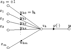
The model they proposed is deliberately simple. A unit receives several input signals (think of them as numbers). It combines these inputs by weighting each one and adding them together — an aggregation step, drawn in the diagram below as a summation Σ. Then it applies a threshold condition: if the weighted sum is large enough to cross some threshold, the unit “fires” and outputs 1; otherwise it stays quiet and outputs 0.

Why is this so significant? Because with just a handful of such units you can implement elementary logic — AND, OR, NOT. For example, an AND unit could fire only when both its inputs are on; an OR unit fires if any input is on. The diagram above walks through exactly this structure: weighted inputs feed into a summing circle, the sum passes to a threshold box, and finally you get a binary 0/1 output.

The figure labeled “generalized artificial-neuron structure” shows the same idea in slightly different form — again emphasizing that input → aggregation → threshold → output is all there is to this unit.

Two warnings keep your understanding precise:

• It is not a complete biological neuron. Real neurons have timing, chemical effects, decay and much more. The McCulloch–Pitts model keeps only the computational skeleton — which is exactly why it was useful: abstraction removes distracting detail to expose logic.
• By itself it is not yet a learning procedure. Crucially, the 1943 paper described what such units compute, but said nothing about how you would automatically find good values for the weights and threshold. In other words: “specify what the unit computes” and “explain how suitable parameters are obtained” were treated as separate tasks — and only later work (the perceptron) tackled that second task of learning.

Hold onto this distinction, because it defines a recurring theme in AI history: having an architecture for representing knowledge is one thing; having an algorithm for acquiring the parameters from data is quite another. McCulloch–Pitts gave us the first half.

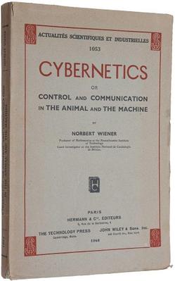
The mathematician Norbert Wiener coined the term cybernetics (from a Greek word for steering or piloting) in his 1948 book, whose first edition is pictured below. Cybernetics is the study of communication and control — especially how systems regulate themselves through feedback. It grew directly out of Wiener’s wartime work on anti-aircraft aiming, where you must keep predicting and correcting a moving target.

The core pattern, which you already experience daily, works like this:

1. A system has some desired condition — a goal (e.g., “room at 21 °C” for a thermostat).
2. It takes an action or sends a signal toward that goal (turn the heating on).
3. It observes the actual result of its action (reads the temperature).
4. It compares the observed result with the desired condition.
5. If there is a difference, it adjusts its next action to reduce that difference (turn heating up or down), then repeats.

The power of this loop — observe → compare → adjust → repeat — is that no one needs to pre-compute the perfect sequence of actions. The system keeps correcting itself in real time, so it can cope with disturbances (someone opens a window) without being told about them in advance.

Wiener’s key insight was that this same feedback principle appears everywhere: in thermostats and cruise control, but also in biology — how an animal reaches for food or keeps its balance, how your body regulates temperature. Cybernetics therefore forged a bridge between biological behavior and engineered machines by pointing out they share one unifying mechanism.

For AI specifically, cybernetics contributed a subtle but profound shift of perspective: intelligent behavior can be organized as an ongoing interaction with an environment, rather than only as a fixed calculation from a static input to a final output. A thermostat never “finishes”; it continuously participates in the world. This idea — agents sensing, acting and adjusting over time — is the direct ancestor of modern robotics and reinforcement learning, where decisions depend on feedback received along the way instead of being fully determined at the start.

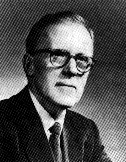
The psychologist Donald Hebb, pictured below, contributed one of the most influential ideas in all of learning theory: a hypothesis for how experience could physically change a network. In his 1949 book he proposed what we now call Hebbian learning: when two connected units are active at roughly the same time, repeatedly, the strength (weight) of the connection between them is increased.

You have almost certainly heard this idea compressed into a catchy slogan — “neurons that fire together wire together.” It appears everywhere in popular science. But you should know two things about it: first, that exact phrase is not a verbatim quote from Hebb’s book; it is a later paraphrase coined to summarize his idea. Second, and more importantly for your understanding, the slogan is only a shorthand — it captures the flavor of Hebbian learning but not its full content or limitations.

The deep significance of Hebb’s rule was that it offered a completely unsupervised mechanism for change: connections strengthen simply as a result of which patterns happen to occur together. No external teacher, no comparison against correct answers — just co-activation over time. This connects experience directly with changes in the network’s effective internal structure; things that tend to go together (seeing a flame and feeling heat) become more strongly linked.

To place Hebb correctly, contrast him with what came later:

• Hebbian learning: connections change based purely on co-activity. There is no notion of right or wrong — the pattern simply gets reinforced if it repeats.
• Supervised error correction (e.g., the perceptron rule you’ll meet soon): first compare a prediction with an actual target/answer, then adjust weights specifically to reduce the resulting error. Here learning is driven by being told what was correct.

These are genuinely different kinds of learning. Hebb gave us “experience reinforces whatever happens together”; supervised methods give us “feedback on mistakes drives correction.” Modern AI uses both, sometimes combined.

Finally, tie this back to the previous section: remember that McCulloch–Pitts described what a neuron computes but supplied no way to learn its parameters. Hebb’s rule was precisely an early answer to that missing half — one possible mechanism for how connection strengths could be obtained and updated from experience, even if (as his critics noted) the bare slogan is not yet a complete specification of all neural learning rules.

The fourth chapter brings everything together. By the mid-1950s all the pieces from earlier chapters were in place — statistical tools for reasoning with evidence, a theory of computation defining what machines could do, and biological inspiration for neuron-like units that could learn. In this decade those threads finally converged into something with an explicit name: artificial intelligence.

The chapter covers four directions that the young field pursued more or less at once:

• Reasoning and search. Programs like Logic Theorist tried to prove mathematical theorems by systematically exploring valid steps of logic, treating a problem as a search through possibilities. This is the “symbolic” side of AI — reasoning with explicit rules and symbols.
• A common name and agenda. The 1956 Dartmouth workshop gave the field its identity: an agreed-upon term (“artificial intelligence”) and an ambitious research program covering language, abstraction, learning and self-improvement.
• Learning from examples. Frank Rosenblatt’s perceptron showed a machine that genuinely adapted, adjusting itself based on data rather than following fixed instructions — the “learning” side of AI. Learning and hand-crafted reasoning developed together, not one after the other.
• Tools for symbolic work. John McCarthy’s Lisp made it convenient to manipulate symbols (not just numbers), which suited logic, language and recursive programs; meanwhile Arthur Samuel’s checkers program demonstrated learning from experience by playing against itself.

The early results were striking but restricted: each demonstration worked only within a narrow domain. What excited the field was not any single feat but the hope that reusable computational principles — search, representation, learning, feedback — might support far broader forms of intelligent behavior than any one program yet showed.

This is also your first chance to see both main strands of AI side by side: symbolic reasoning (explicit rules and logic) and learning-based approaches (adjusting parameters from data). Throughout history these two have complemented, competed with, and borrowed from each other — a tension we will watch develop in later parts.

This section gives you a compact overview of the early landmarks that together defined what AI was going to be. Notice how they deliberately combine two different philosophies:

• The reasoning/search side. Logic Theorist (Newell, Shaw & Simon) and its successor General Problem Solver attacked problems by explicit logical deduction and by search — exploring a space of possible states toward a goal. These programs treated intelligence as careful symbolic manipulation according to rules.
• The learning side. Rosenblatt’s perceptron learned to separate data into categories purely from examples, adjusting its weights when it made mistakes. Meanwhile Arthur Samuel taught checkers to improve through experience — famously by playing thousands of games against itself — rather than prescribing every move in advance.

These two threads also relied on different enabling tools: the reasoning programs worked best with a way to represent and manipulate symbols (which is where Lisp came in), while the learning systems needed a mechanism for changing decisions based on data or feedback.

The single most important historical point here — easy to miss if you imagine history as neat stages — is that learning-based and symbol-based approaches developed together from the very beginning. The field did not first do “pure reasoning” and then later discover “machine learning”; both were present at the birth in 1955–57. Researchers explored them side by side, sometimes combining ideas across the two camps.

So when you study machine learning as a distinct topic, remember it was never an afterthought bolted onto AI — it is one of the field’s founding strands, and this section shows precisely where its early landmarks (perceptron, checkers) sit alongside the reasoning pioneers (Logic Theorist, General Problem Solver).

In 1955–56, Allen Newell (a computer scientist), J. C. Shaw and Herbert Simon built one of the very first AI programs: Logic Theorist. Its goal was nothing less than proving mathematical theorems — but not by doing clever human mathematics; instead it showed that theorem-proving could be recast as a search problem.

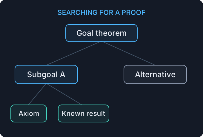
The key reframing is this: think of all the true statements and rules of logic you are allowed to use. From any starting statement, applying one valid rule gives you another statement (a deduction). Proving a theorem means finding a chain of such deductions that ends at your desired conclusion — like threading a path through a maze where each corridor step is an allowed logical move.

The figure below (“a schematic search through goals and known results”) illustrates this organization. Please note it is exactly that — a schematic, meant to show how such searches are structured, not a literal rendering of one particular proof.

Logic Theorist had two crucial ingredients:

1. A representation. Theorems and rules must be written down in some formal notation the program can manipulate — this is what it means for an intellectual task to become “represented” inside a machine.
2. A strategy for choosing which deductions to try next. Because there are far too many possible moves, the program needed heuristics (rules of thumb) to pick promising paths rather than wander randomly. This guided selection is the difference between intelligent search and brute-force enumeration.

The successor project, General Problem Solver, pushed this further with an idea called means–ends analysis: describe both your current state and your goal, then identify the most important difference between them, and pick an action that reduces it — repeatedly shrinking the gap until you arrive at the goal. (You can recognize this as a general strategy humans use all the time when planning.)

The lasting contribution of these programs was conceptual: they showed that “intellectual” tasks like proving theorems could be broken into representation + legal operations + search strategy, and thereby become computable. Historically it is reported that Logic Theorist proved several of Russell and Whitehead’s classic logic theorems — a striking early result. Treat this proof count as a reported historical claim, not an experiment you need to reproduce here; the important lesson is architectural, about how reasoning was turned into search.

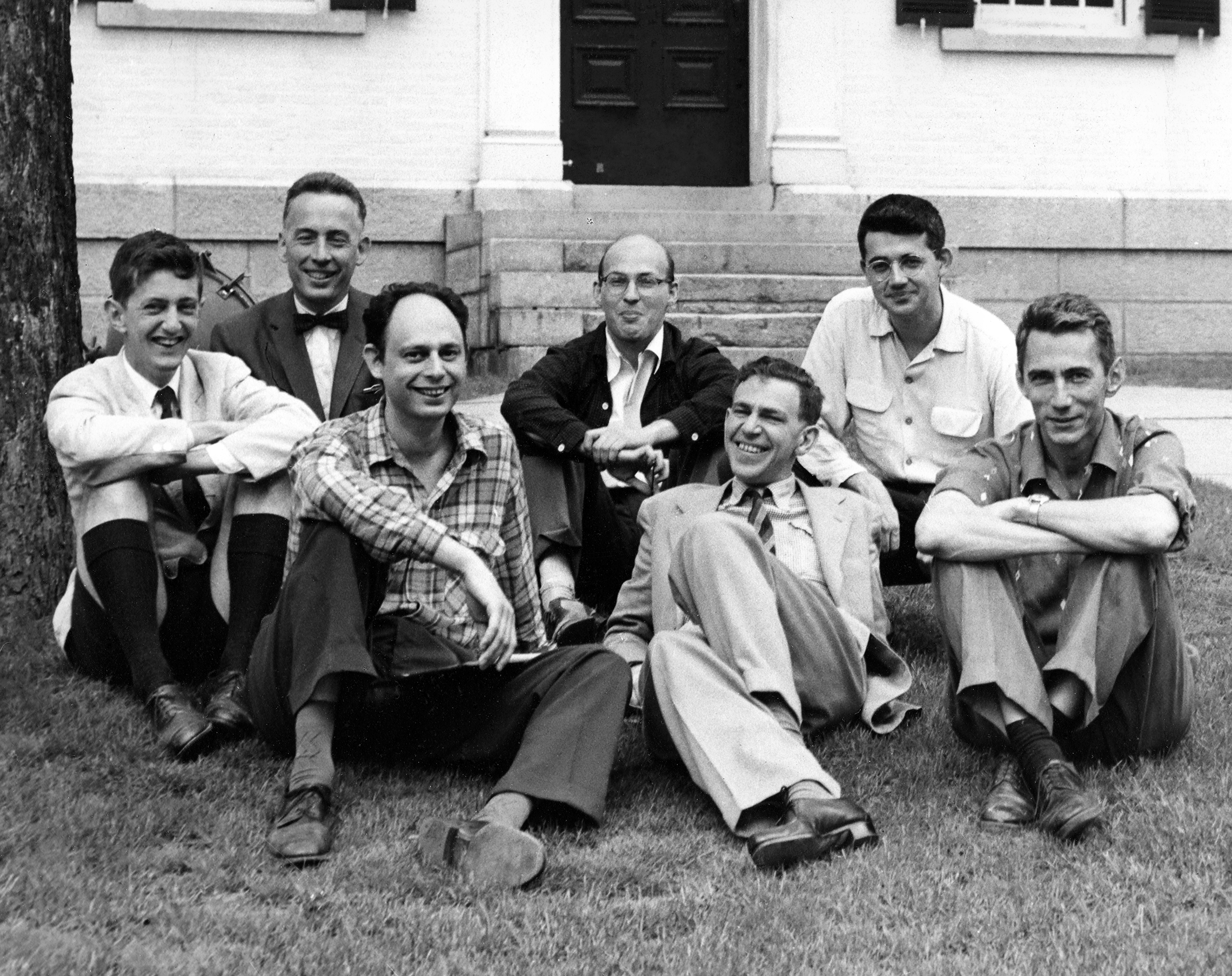
The moment the field received its name — and its grand agenda — was a proposal written in 1955 and followed by a summer research project held at Dartmouth College in 1956. Its four authors were John McCarthy, Marvin Minsky, Nathaniel Rochester and Claude Shannon, and remarkably, the title of the proposal already contained the phrase “artificial intelligence” a year before the workshop took place.

The proposed study was breathtakingly ambitious: it planned to investigate how machines could be made to use language, form abstractions and concepts, solve kinds of problems reserved for humans, and improve themselves. The organizers openly predicted that progress in these areas over “an intensive 2 month, 10 man study” might produce a machine capable of learning or forming abstractions — a famously optimistic forecast.

It is essential to understand what the Dartmouth project did and did not do:

• What it did: It provided an influential, unifying name for the field (“artificial intelligence”) and a shared research agenda that pulled together scattered efforts under one banner. The photograph above shows some of the participants who gathered for the 1956 workshop — an important community-building event.
• What it did not do: It did not invent every underlying idea. All the core concepts — Bayes’ theorem, regression, Turing machines, artificial neurons, Hebbian learning — already existed and were developed elsewhere over decades. The workshop organized and branded these efforts; it did not conjure them from nothing.

The original proposal is worth reading for a striking reason: it records, in the organizers’ own words, both their soaring expectations and their honest acknowledgment of obstacles. Seeing how they framed machine intelligence “in 1955” — what seemed within reach and what they knew was hard — gives you invaluable perspective on how far (and sometimes how little) the field has moved.

For your studies, Dartmouth matters mainly as the symbolic birth certificate: after 1956 there existed a recognized community with a name, a set of core questions, and an agenda that would shape AI research for decades to come.

The perceptron, built by psychologist Frank Rosenblatt in the late 1950s, was a genuine turning point: it combined two earlier ideas into one working learning machine. Recall that McCulloch–Pitts told us what an artificial neuron computes but gave no way to learn its parameters; Hebb suggested connections could strengthen through co-activity but had no notion of error or correctness. Rosenblatt’s perceptron added the missing ingredient — learning from mistakes.

The architecture is simple: a set of inputs, each multiplied by a weight and summed (just like our neuron), then passed through an activation that decides between two output categories. Geometrically, you can think of it as drawing a straight line (a linear separator) in the space of inputs — all points on one side get classified “A,” all points on the other side “B.”

The breakthrough was the learning rule. In the supervised formulation you will study in detail later in this course, training works like this: feed an example through the perceptron to get a prediction, compare it with the true answer (the target), and if there is an error, adjust the weights and bias slightly so that next time the same input would be classified correctly. Repeat over many examples until mistakes stop.

Because this rule updates only when there is a mistake, and adjusts toward the correct answer, it differs from Hebbian learning in an essential way — Hebb strengthens purely on co-activity with no concept of right or wrong. You should also keep it distinct from another common method called the delta rule, which handles smooth (differentiable) error surfaces for squared-error learning; each is a different algorithm for adjusting weights, suited to slightly different settings.

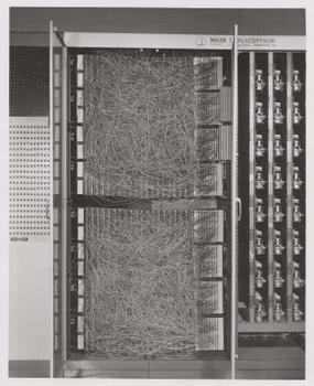
The historical machine photographed above — the “Mark I Perceptron” built in 1958 as an actual physical device with light sensors and motors — makes vivid how seriously researchers took the ambition of learning from data. Yet even this exciting success carried a warning that would surface again: because a single perceptron can only draw one straight-line boundary, its geometry decides what it can represent. Some patterns simply cannot be separated by any single line (you will see classic examples later), which set an important limit on how powerful individual units could be — and eventually motivated stacking many neurons into networks.

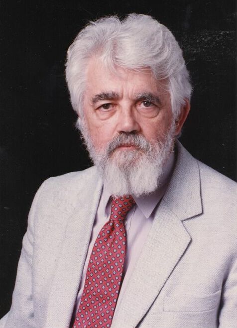
The final landmark of this era is Lisp, a programming language created by John McCarthy (the Dartmouth organizer, pictured below) in 1958. To understand why it mattered, remember the split between the two strands of early AI: learning programs worked with numbers and data, while reasoning programs like Logic Theorist manipulated symbols — logical expressions, rules and language-like structures.

Most programming languages at the time were built around numbers. Lisp was different: it made symbolic expressions — nested lists such as (OR (NOT A) B) representing logical formulas or program code itself — extremely easy to create, combine and rewrite. This turned out to be exactly what reasoning programs needed:

• language processing could treat sentences as symbols;
• logic could represent theorems and rules directly; and
• recursive structures (like “a list can contain lists”) mapped naturally onto the way problems are broken into smaller versions of themselves.

A neat historical point: in Lisp, data and program code look almost identical. A list like (+ 1 2) is just data until you decide to evaluate it as a program that returns 3 — which means a Lisp program can manipulate other programs as if they were ordinary data. That flexibility made it ideal for AI experimentation.

The second half of this section turns to the learning strand via Arthur Samuel’s checkers program, built around the same time (1959). Rather than hand-coding every possible move — an impossible task — Samuel had the machine learn how good positions were by playing many games, including against itself. Over experience it improved its play without a human specifying each decision. This was one of the earliest and most celebrated demonstrations that behavior could improve through experience, not just from being programmed with answers.

Taken together, Lisp and Samuel’s checkers neatly illustrate the two prerequisites every AI system needs:

1. Representation — a useful way to encode your problem (Lisp gave symbolic reasoning its notation).
2. Adaptation — a mechanism for changing decisions in response to evidence or feedback (Samuel’s checkers learned from games it played).

A system needs both: without good representation, there is nothing meaningful to compute; without adaptation, the system can only follow fixed instructions and never improve. This pairing of representation + learning is a lens you can carry through every later chapter — indeed, through all of machine learning.

You have now traced the journey that made AI possible — from eighteenth-century probability, through a precise theory of computation, to biology-inspired neurons and finally to named learning machines in the 1950s. Before moving on, check your understanding against these three core takeaways:

• Explain how evidence can change a belief. Use Bayes’ theorem: you start with a prior degree of confidence, observe new evidence, combine it with how likely that evidence would be under your hypothesis (the likelihood), and arrive at an updated posterior. Give a concrete example — for instance, updating the probability of rain after seeing clouds in the morning.
• Distinguish a test of behavior from a claim about consciousness. Turing’s imitation game is a behavioral evaluation: it asks only whether an examiner can tell machine from human through text. Passing or failing that test says nothing, by itself, about inner experience — so you should be able to separate “behaves as if intelligent” from any claim about what the machine actually feels or understands.
• Connect early learning systems with examples and feedback. Rosenblatt’s perceptron improved its weights when its predictions were wrong (error-driven, supervised). Hebbian learning strengthened connections through co-activity alone. Samuel’s checkers improved by playing games and evaluating outcomes. All are ways experience or feedback changes a system — the essence of machine learning.

Now choose one of these three ideas and explain it in your own words using an example from this part. Teaching it back is the surest way to know you have really learned it — and it is exactly what you will do when you revisit these concepts in later lectures, where Bayes appears again in classification, feedback reappears in reinforcement learning, and neural units grow into deep networks.