History of artificial intelligence · Part 2

Welcome back! In Part 1 we traced the foundations that made artificial intelligence possible: probability as a way to reason under uncertainty, Turing’s precise theory of what computation even is, and early biology-inspired neurons with hints of learning. Those ideas gave AI its birth in the 1950s.

Before continuing into Part 2, make sure you can answer three quick recap questions from where we left off:

• Explain how evidence can change a belief. Use Bayes’ theorem: you start with some prior confidence, observe new evidence, combine it with the likelihood of that evidence under your hypothesis, and arrive at an updated posterior — e.g., raising your rain estimate after seeing morning clouds.
• Distinguish a test of behavior from a claim about consciousness. Turing’s imitation game only evaluates what a machine does (whether a human examiner can tell it apart through text). Passing or failing says nothing, by itself, about whether the machine truly feels or understands anything inside.
• Connect early learning systems with examples and feedback. Rosenblatt’s perceptron adjusted its weights when predictions were wrong; Hebbian units strengthened connections through co-activity; Samuel’s checkers improved by playing games. All are ways experience changes a system — the essence of machine learning.

With those foundations fresh, Part 2 follows what happened after the optimistic birth: how expectations outran reality and triggered AI “winters,” how expert systems brought knowledge back into focus, how neural networks returned and grew into deep learning, how modern generative models emerged, and how recent systems such as Jev return structured decisions for software. The story is one of recurring cycles — excitement, disappointment, then renewal on stronger foundations.

The story of AI is not a smooth upward line — it alternates between bursts of enthusiasm and periods of disappointment, now famously called AI winters. The first such winter came in the late 1960s and into the 1970s. To understand why, you have to appreciate how high expectations had climbed during AI’s optimistic birth a decade earlier.

In the 1950s researchers made genuinely impressive demonstrations: programs that proved theorems from Principia Mathematica, machines that learned simple patterns, systems that played checkers. But these early successes were all confined to narrow, carefully chosen tasks inside very small worlds. It was natural — and in hindsight too easy — for the press, funders and even some researchers to extrapolate wildly: if a program can prove one theorem or learn one pattern, why not soon solve most intellectual problems? The gap between such expectations and what the technology could actually do became enormous.

This first winter teaches an enduring lesson you will see repeated throughout AI history: a restricted technical achievement is not evidence that general intelligence has been solved. Showing that a program can beat a human at checkers tells us something about checkers, not yet about common-sense reasoning or understanding language. Each success deserves celebration — but also honest calibration about how much it actually demonstrates.

One clarification worth keeping straight: this teaching period spans the late 1960s and 1970s as a broad era of reduced funding and enthusiasm, while specific events within it (such as Minsky and Papert’s critical 1969 analysis of perceptrons, which we look at next) are distinct historical moments. The winter was caused by many interacting forces — funding decisions, hardware limits and unmet promises — not by any single book or theorem alone.

A key technical trigger for disillusionment was a landmark 1969 book by Marvin Minsky and Seymour Papert, titled simply Perceptrons. Its most famous contribution was a careful mathematical analysis of what single perceptron units can and cannot learn — and the answer, as they showed rigorously, is quite limited.

The accessible example everyone remembers from that work is the XOR problem. Imagine two input signals, each either 0 or 1. XOR (exclusive-or) asks: “are the two inputs different?” It should output 1 when exactly one of them is on, and 0 when both are equal. If you plot this as four points in a square — the corners representing (0,0), (0,1), (1,0), (1,1) — you find that the matching labels sit on opposite corners. There is no single straight line you can draw across the plane that puts all 0-labelled points on one side and all 1-labelled points on the other. A perceptron, which classifies by drawing exactly such a straight boundary, therefore simply cannot represent XOR correctly, no matter how its weights are tuned.

Minsky and Papert’s analysis had enormous consequences: it showed that early neural networks — those built from just one layer of these units — were fundamentally limited to problems whose classes could be separated by a straight line. Combined with the general mood of unmet expectations, this helped deflate enthusiasm for the neural approach.

But two caveats keep your understanding accurate and historically fair:

• A representation limitation is not proof that all neural systems fail. The result applied to single-layer perceptrons. Adding more layers of units changes what can be represented — a multilayer network can indeed solve XOR — although it makes the question of how to train such networks harder (that challenge was only solved convincingly later, with backpropagation).
• The book did not cause the whole winter on its own. The period’s downturn came from a combination of hardware limits, funding decisions, inflated expectations and mixed results across many research programs. A broad change in an entire field is never the work of one theorem alone — even so influential an analysis as this one.

The diagram above therefore motivates two separate questions you should always keep apart when studying learning systems: can a model express a solution? (a representation question) versus is there a procedure that can find good parameters? (a training/learning question). A perceptron fails the first for XOR; later networks solved it but faced new difficulties on the second.

In XOR, points with the same target occupy opposite corners, so one straight line cannot separate the two classes. This is a limitation of that representation, not proof that all neural systems fail on the task. More expressive architectures change the representational question, although their training may be harder. The diagram therefore motivates two separate questions: whether a model can express a solution and whether a procedure can learn suitable parameters.

The 1980s brought a major shift in strategy. Instead of trying to build systems that reason about everything, many researchers and companies focused on the opposite extreme: capturing one expert’s hard-won knowledge within a very narrow specialty, then turning it into a computer program that could give reliable advice in that domain.

These programs became known as expert systems. The core idea was to encode specialist knowledge explicitly — usually as rules of the form “IF condition THEN conclusion” — so that the machine could reason the same way an experienced human professional does. Rather than learning from data (as perceptrons tried to do) or searching enormous spaces, expert systems consulted a carefully assembled storehouse of knowledge.

The approach had real appeal and genuine successes: in medical diagnosis, chemical analysis and equipment configuration, such systems could capture decades of human expertise and make it available anywhere. For a time they became AI’s most commercially successful and widely deployed technology — a striking contrast to the disappointment of the preceding winter.

But expert systems also exposed two hard truths that shaped everything after them:

• The value of domain expertise. Encoding what specialists actually know proved remarkably powerful; knowledge really is central to intelligent behavior, not something you can skip.
• The difficulty of maintaining it. Acquiring accurate rules from experts was slow and painstaking. And once a system grew large, keeping thousands of rules mutually consistent — adding new ones without breaking old conclusions, handling unusual cases — became an enormous maintenance burden in its own right.

So the expert-systems era taught AI that useful intelligence depends on far more than having a clever algorithm: you also need domain knowledge, careful organization and ongoing upkeep. These lessons remain relevant today whenever we ask how hard it is to build and maintain systems meant to match human expertise.

The expert-systems era produced several landmark systems you should be able to name and contrast:

• DENDRAL (1960s–70s): inferred the chemical structure of organic molecules from mass-spectrometry data. It showed that a program could outperform individual chemists at specific, well-defined identification tasks.
• MYCIN (1970s): diagnosed bacterial infections and recommended antibiotic treatments using a large set of medical rules with associated confidence factors. Although never widely used in practice, it became the classic research example for how to structure knowledge-based reasoning.
• R1 / XCON (~1980): configured complex DEC computer systems — deciding which components fit together and ordering them correctly. It was one of the first expert systems deployed commercially on a large scale, saving real time and money.

Alongside these successes ran an even more ambitious project: Japan’s Fifth Generation Computer Systems program (1982–92). Rather than encoding expertise in software alone, Japan aimed to build entirely new kinds of computers — highly parallel machines designed around logic programming and artificial intelligence — that would leapfrog the general-purpose hardware then on the market. The project galvanized AI investment worldwide for a decade.

The deeper lesson across all these developments is this: AI depends on more than an abstract algorithm. A brilliant reasoning method means little if you cannot acquire good knowledge, organize it coherently in software, afford the hardware to run it, and keep its scope realistically bounded. Whether any approach becomes genuinely useful outside a small demonstration hinges on these practical factors every bit as much as on mathematical cleverness.

In hindsight, the Fifth Generation’s specific bet — that specialized parallel logic machines would dominate AI — was overtaken by increasingly powerful general-purpose hardware running ever-better software. That outcome illustrates how even technically sound visions must respond to changing costs and competing ways of doing the same job.

Let’s look inside an expert system to see exactly how it works. Every such program is built from two essential parts:

• A knowledge base: a collection of facts and rules supplied by human experts, written down in some structured notation.
• An inference mechanism (inference engine): the software that takes new observations about a specific case, applies the stored rules to them step by step, and draws conclusions from what it knows.

The simplest way these two parts interact is through if–then chains. Suppose we observe some condition (say, “the patient has a high fever”). This matches the IF-part of one rule: IF high fever AND other symptoms THEN suspect infection. The conclusion (“suspect infection”) becomes new information that can itself satisfy the IF-part of another rule — IF suspected infection THEN order more tests — and so on. Each deduction opens the door to further deductions, letting a relatively small set of rules generate quite complex reasoning paths.

In this lecture you may see such an inference chain drawn as a tree or diagram in a medical setting (symptoms leading to diagnoses). Treat it exactly as what it is: a schematic illustration, built for teaching how rule-chaining works. It is not a clinical decision tool, and no patient should be diagnosed by it.

The general lesson about expert systems applies far beyond medicine: the hard part of keeping such a system useful over time is maintaining its rules — making sure they stay accurate, remain mutually coherent (new rules don’t contradict old ones), and grow sufficiently complete as unusual cases and new knowledge accumulate. Every era of AI confronts some version of this maintenance problem.

A final historical clarification: the expert-system tradition is broader than medicine alone. DENDRAL inferred chemical structures starting in the 1960s; MYCIN handled medical consultation in the 1970s; R1/XCON configured computer systems around 1980. Medicine was an early and influential application area, but by no means the sole origin of expert systems.

Japan’s Fifth Generation Computer Systems project (1982–92) was one of history’s most dramatic bets in computing: a national, decade-long program to build machines purpose-built for artificial intelligence. To see why it matters and what went wrong, consider the two competing strategies it highlighted.

• The specialized bet. Instead of using ordinary computers programmed with software, the Fifth Generation planned dedicated parallel, logic-oriented hardware — thousands of processors working together on logical reasoning at once. The idea was that such machines would make AI fast and natural enough to dominate everything else.
• The general-purpose alternative. Meanwhile, ordinary computers kept getting dramatically faster, cheaper and more capable every single year. Software running on this mainstream hardware could do the same AI work without any special machinery — and with far less risk, since it leveraged an enormous existing market.

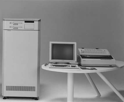
The photograph in this lecture shows one artifact of that effort: a dedicated inference workstation, a machine engineered specifically to execute logical deduction quickly. It stands as physical evidence of how seriously researchers took the specialized-computing vision.

In the end, general-purpose hardware won: it improved so fast and cost so little that Japan’s parallel logic machines could not compete on price or practicality. The lesson is worth stating carefully because it is easy to overlearn:

• It does not mean specialization always fails — dedicated chips can be enormously valuable (graphics cards for modern deep learning are exactly such a success story).
• Rather, the real lesson is that a technical vision must keep responding to changing practical requirements, implementation costs and competing ways of doing the same work. A bet on one paradigm carries risk if it ignores how fast alternatives improve.

The Fifth Generation project was not a total loss — it stimulated worldwide AI research and funding for years — but its specific hardware prediction was overtaken by the relentless march of general-purpose computing.

After the pessimism of the first AI winter — especially Minsky and Papert’s sharp critique of single-layer perceptrons — one might expect interest in neurons to have died out. Instead, a movement called connectionism came back stronger from the 1980s onward.

The word “connectionist” signals its core belief: intelligence should be built not from explicit symbolic rules but from large numbers of simple connected units whose strengths (weights) are learned. The key advance was to move decisively beyond a single threshold unit. Researchers introduced richer architectures and better training methods that overcame the limitations identified in the 1960s:

• Spatial hierarchies. Networks organized so they detect simple local features first and combine them into more complex patterns, mirroring how visual processing appears to work. (The Neocognitron and modern convolutional networks.)
• Recurrent memory. Networks whose connections loop back on themselves, giving the system a kind of state or memory over time rather than just reacting to one input in isolation. (Hopfield networks.)
• Efficient gradient calculations. A practical method — backpropagation — for computing how every internal weight should change so that multi-layer networks could actually be trained. (Rumelhart, Hinton and Williams.)

Notice that each of these addresses a different part of the overall challenge: hierarchies tackle representation, recurrent connections tackle memory/dynamics, and gradient methods tackle training. Only by combining all three could neural systems become genuinely useful. This chapter walks through them one at a time, so you can see exactly what problem each solved.

This section gives you an overview of three distinct contributions from the connectionist revival, so you can appreciate how each solved a different problem:

• The Neocognitron and later convolutional networks organized visual processing hierarchically. Instead of treating every pixel independently, they first detected tiny local features (edges, corners), then combined those into slightly larger patterns, layer by layer. This hierarchical structure — built to tolerate small shifts in position — addressed the hard problem of representation: how should a system internally describe what it sees?
• Hopfield networks explored recurrent dynamics and associative memory. Their connections loop back, so the network’s state evolves over time. Stored patterns act as attractors: feed in a noisy or partial version of a memory and repeated updates pull the whole state toward the nearest complete memory — rather like recognizing a face from an old, faded photograph.
• Backpropagation provided a way to efficiently calculate derivatives through multilayer computations. It answered the training question left open since Minsky and Papert: how do we compute how much each weight deep inside a network should change when the output is wrong? By propagating the error backward layer by layer, it made gradient-based learning practical for multi-layer networks.

So these three contributions respectively address representation (how to structure features), memory/dynamics (how state can evolve over time) and training (how to adjust parameters from data). Together they reinforced a pivotal idea that would define modern AI: rather than having humans hand-design every feature and decision rule, a system could learn useful internal representations for itself. That single shift — from specifying the features by hand to letting them emerge from data — is arguably the most important conceptual change in this entire history.

The Neocognitron, proposed by Kunihiko Fukushima in 1980, is the clearest intellectual ancestor of today’s convolutional neural networks (CNNs) — the models behind modern computer vision. Its key insight was a question about how to recognize objects even when they shift around: how can a visual system detect “there is an edge here” no matter whether that edge appears at one position or two pixels over?

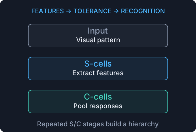
Fukushima’s answer introduced a hierarchy of alternating cell types:

• S-cells: simple cells that respond to specific local features (like an oriented edge) in a small patch of the image.
• C-cells: complex cells that combine responses from nearby S-cells, giving tolerance to position changes. A feature detected slightly to the left or right still triggers the same higher-level response.

Stacking these layers means simple local features are assembled into progressively more complex patterns — edges become corners, corners become shapes, shapes become objects. This is exactly the organizing principle you will see again in modern CNNs: local feature extraction plus a mechanism for position tolerance, repeated hierarchically.

The historical Neocognitron and later convolutional networks share this spirit but are not identical. Modern CNNs (starting with LeCun and collaborators’ 1989 handwritten-ZIP-code recognizer) combined that architectural idea with supervised training via backpropagation. Fukushima’s earlier model already learned from data through self-organization; the later advance was not the introduction of learning itself. So when you look at a hierarchy diagram of processing stages, read it as distinguishing layers in an architecture — not as claiming Fukushima’s specific implementation equals every modern convolution/pooling operation.

The continuing principle that survived intact is the most valuable one: more complex visual patterns can be assembled from simpler local responses. Whether you are recognizing handwritten digits or objects in photos, starting with small reusable detectors and building them up hierarchically turns out to be an enormously effective design — one this 1980 model anticipated years ahead of its time.

The Hopfield network, introduced by physicist John Hopfield in 1982, took neural networks in a strikingly different direction — toward memory and dynamics. Where most classifiers take one input, produce one output and stop, a Hopfield network’s connections loop back on themselves (they are recurrent). That single architectural choice changes everything: the state of the network keeps updating again and again, evolving over time.

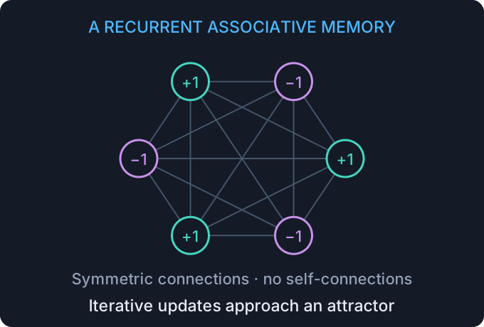
Think of it this way. First you store a set of patterns in the network by setting its weights appropriately — these become your memories. Later, when you present an incomplete or noisy version of one pattern (say, a picture with half the pixels missing), the network does not just output something and stop: it repeatedly updates until its state settles. Because stored patterns act as attractors, the dynamics naturally pull any nearby starting point toward the nearest complete memory.

This is associative or “content-addressable” memory: you retrieve a full memory by supplying only part of it, much as the smell of an old place can trigger a whole recollection. The key conceptual shift is that the dynamics themselves are part of the computation. A Hopfield network’s answer emerges from how its state evolves over many updates — which is why judging it after just one update would completely miss how it works.

The mathematical details (for those who want precision) are elegant: with symmetric connections, no self-connections and asynchronous threshold updates, the network has an energy function that never increases. Each update moves the state downhill in energy until it reaches a stable minimum — which is exactly how physicists like Hopfield think about systems settling into low-energy states. (A consistent rule keeps the state unchanged when there is zero local field.) The schematic below makes these feedback connections visible.

• A useful caution: if you instead update all units synchronously, the system can cycle forever without settling — so implementation details genuinely matter.
• And stored patterns are not guaranteed to be recalled correctly for arbitrary weights or when too many memories overload the network. Capacity has limits, as with any memory device.

Hopfield networks may no longer dominate modern AI, but they established a profound idea: that computation can happen through the temporal evolution of a recurrent system — an idea that reappears in later sequence models and neural dynamics research.

Backpropagation (short for “backward propagation of errors”) solved the training problem that had haunted multilayer networks since Minsky and Papert: how do you figure out which weight to change, by how much, when the network has many layers between input and output?

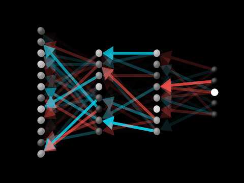
The idea rests on a calculus tool called the chain rule. The network’s output feeds into a measure of error (a loss) that tells us how wrong its prediction was. That loss depends on the last layer’s weights; those depend on the previous layer’s outputs; those in turn depend on earlier layers — all the way back to the input. The chain rule lets you compute, for every internal weight, exactly how much a tiny change to that weight would affect the final error: these sensitivity values are called gradients. “Backpropagation” is the clever, efficient algorithm that works out all these gradients by passing information about the output error backward through the network, one layer at a time.

Once you have those gradients, an optimizer (such as gradient descent) uses them to nudge each weight in the direction that reduces the loss. It is important to keep these two operations distinct:

• Gradient calculation (backpropagation): computes how much each parameter influences the error.
• Gradient descent / optimization: decides how to change the weights using those computed gradients, usually in small repeated steps until the loss stops improving.

In other words, backpropagation is not itself the learning rule — it supplies the information (the gradients) that a separate optimizer then uses. The lecture highlights the hugely influential 1986 paper by Rumelhart, Hinton and Williams (Learning representations by back-propagating errors) which popularized this approach; the accompanying video visualizes how an error at the output propagates its influence to earlier parts of a multilayer computation.

A fair historical note: while 1986 made backpropagation famous, it did not invent every underlying idea about differentiation and gradient-based training — those had older roots. Backprop’s real contribution was turning them into a practical method for deep networks at scale, thereby unlocking the modern era of neural learning.

Just as in the first winter, enthusiasm for neural networks cooled again — this time roughly in the late 1980s and early 1990s. But it is crucial to see that this “second AI winter” was not simply a repeat of the first, nor caused by any single event.

Two separate threads were happening at once:

• Difficulties in neural training. Although backpropagation had made multilayer networks trainable in principle, they remained hard to use well. Training was slow on available hardware, and deeper networks suffered from problems like the vanishing-gradient effect (which we examine shortly), where the learning signal faded away across many layers. Disappointing practical results dampened enthusiasm for neural approaches.
• The rise of alternative statistical methods. Meanwhile other families of techniques — kernel-based support-vector machines and tree ensembles — were proving very effective, easier to train and often just as accurate on real problems without all the fiddly tuning. Many researchers rationally shifted their attention there.

Two lessons keep this period in perspective:

1. A limitation of one approach redirects research effort — it does not stop work across the whole field, nor render every earlier idea irrelevant. The neural toolkit shrank in popularity but never vanished; a community kept refining it quietly until conditions (more data and compute) improved.
2. The “winter” was as much about commercial and funding setbacks, inflated expectations and market disappointments as about any technical result. It would be wrong to date an entire commercial downturn by a single 1991 technical paper on gradient behavior; the two are distinct kinds of events.

The broader pattern across AI history is now clear: research enthusiasm rises, bumps into hard limits (technical or financial), cools — but work never truly stops. The next section shows how specific technical challenges like vanishing gradients pushed some researchers toward alternatives that would remain important tools even long after deep learning returned.

During the late 1980s and early 1990s two kinds of development unfolded together: a specific technical obstacle inside deep learning, and a broader shift toward alternative methods. Understanding both helps you see why this period is called a “second winter” for neural networks yet was actually quite productive overall.

• The vanishing-gradient problem (technical). To train a network with many layers or recurrent loops, backpropagation must push learning signals backward through every transformation. When those transformations repeatedly shrink the signal — mathematically, when derivatives are small and get multiplied together across layer after layer — by the time information reaches early parameters it has become so tiny that training effectively stalls there. We look at this in detail next; for now note it made some deep and recurrent models genuinely hard to train on the hardware of the day.
• Kernel methods and tree ensembles (alternative routes). Rather than fighting these difficulties, many researchers turned to approaches that sidestepped them. Kernel-based support-vector machines found powerful nonlinear boundaries without needing many layers; decision-tree forests aggregated many simple models into strong predictors. These were often easier to train, required less tuning, and delivered excellent results on real problems.

The crucial historical point is to keep these technical developments separate from the broader commercial and funding circumstances of the second AI winter. A mathematical difficulty in training deep networks explains why some methods lost popularity — but it does not by itself explain a market collapse or budget cuts, which had their own causes (unmet business promises, hype cooling). Both stories matter, and conflating them produces a misleading history.

Finally, notice that “winter” is a simplification. Research continued throughout; the alternative methods developed in this period — SVMs, random forests — did not disappear when deep learning returned. They remained part of every practitioner’s toolkit. Periods we call winters were actually times of real methodological progress that later proved essential.

The vanishing-gradient problem, analyzed formally by Sepp Hochreiter around 1991, explains why deep and recurrent networks were so hard to train during the second winter. To understand it intuitively, recall how backpropagation works: a learning signal (based on the output error) travels backward through the network, passing from layer to layer, telling each weight how much to change.

The trouble is that at every step along this backward journey, the signal gets multiplied by derivative values — numbers describing how strongly one unit’s output changes another. If those derivatives are typically smaller than 1 (which happens with common activation functions), then multiplying them again and again across many layers makes the signal shrink exponentially. By the time it reaches the early layers near the input, the gradient has become essentially zero.

The consequence is clear and serious: early parameters receive almost no update during training, even when the output error genuinely matters. The network’s earliest layers essentially fail to learn from data, so a deep network behaves more like it has far fewer effective layers than intended — undermining exactly what made “deep” networks appealing.

But keep this problem in proper perspective with two points:

• It is an optimization difficulty, not a universal impossibility result. Vanishing gradients mean gradient-based training struggles under certain conditions. They do not prove deep learning can never work. Later advances — better activation functions (like ReLU), smarter weight initialization, residual connections and normalization — were specifically designed to keep signals flowing through many layers, and they largely tamed the problem.
• The behavior depends on choices. Whether gradients vanish badly is influenced by architecture depth, the choice of activation function, how weights are initialized and other design decisions. It was never an iron law that every deep network must fail to train.

A final historical caution: while vanishing gradients contributed to the decline in enthusiasm for neural networks, it would be too narrow to blame this one technical issue as the sole cause of a broad commercial and funding downturn. Real history again mixes technical limits with expectations and economics — an interplay you will see repeated at every major turning point.

While deep networks struggled with vanishing gradients, other families of methods flourished — collectively giving researchers powerful new tools that did not require training many layers. The two most influential were kernel-based support-vector machines (SVMs) and tree ensembles, each solving a different problem.

• Kernel methods / SVMs. A support-vector machine finds a boundary that separates classes with the widest possible margin between them. Its power comes from a trick called the kernel: instead of explicitly computing points in a high-dimensional feature space (which could be impossibly expensive), the algorithm only ever needs to compute similarities between pairs of inputs — and certain similarity functions (“kernels”) implicitly correspond to very rich feature spaces. This lets an SVM draw nonlinear boundaries that would otherwise require many layers or hand-built features.
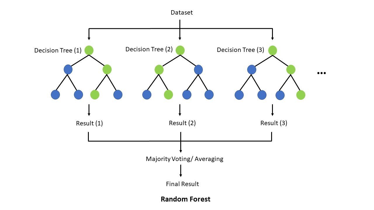
• Tree ensembles / random forests. A single decision tree splits data into regions using a sequence of yes/no tests, and is delightfully easy to read (you can literally inspect the branches). But individual trees are often unstable. Ensembles fix this by training many slightly different trees and aggregating their predictions — for example, each tree votes on the class. The collection (a “forest”) is usually far more accurate than any single tree.

The two approaches embody opposite philosophies about interpretability: one decision tree can be inspected and explained by hand, whereas a large forest’s aggregate prediction is harder to trace back through hundreds of trees — less directly interpretable, though often much stronger.

Key historical milestones anchor this era:

• 1992: Boser, Guyon and Vapnik introduced kernel SVMs (extending earlier margin-based ideas).
• 1995: Cortes and Vapnik formalized the soft-margin SVM, which tolerates a few errors rather than requiring perfect separation.
• 1995: Tin Kam Ho proposed random decision forests; 2001: Leo Breiman’s “random forest” made them practical and widely known.

The most important takeaway is that these methods expanded the machine-learning toolkit rather than replacing every neural or symbolic approach. Real-world AI, then as now, benefits from having many complementary tools — and when deep learning surged back in 2012, SVMs and forests remained valuable options right alongside it.

Around 2006 onward, conditions finally aligned for a dramatic revival — this time so powerful it is called deep learning, and its arrival marked the start of modern AI. To understand why it succeeded now when earlier neural efforts had stalled, you must see that several ingredients came together at once, each reinforcing the others:

• Large datasets. The internet produced vast collections of labeled examples — millions of images with known categories, huge corpora of text. Learning systems thrive on data; deep networks in particular need enormous amounts to discover useful representations rather than just memorize training cases.
• Greater computing capacity. Graphics processing units (GPUs), originally built for rendering video games, turned out to be spectacularly well suited to the highly parallel arithmetic that neural networks require. Training a large network dropped from taking weeks or months on ordinary CPUs to days or hours on GPUs.
• Improved training techniques. Better activation functions (notably ReLU), smarter weight initialization and other practical tricks overcame many of the problems — like vanishing gradients — that had limited earlier deep networks. The math improved, but crucially it became usable at scale.

The most important conceptual lesson is that these factors reinforced one another: more data motivated deeper models; faster hardware made those deeper models feasible to train; better training methods let them actually learn from the larger datasets. It would be a mistake to credit deep learning’s rise to any single ingredient — not just “more data,” nor only “bigger networks,” nor solely “faster computers.” Progress came precisely from how they amplified each other.

This virtuous cycle — more data, more compute, better algorithms feeding back on one another — is the engine that has driven AI forward ever since. Keep it in mind as we look at ImageNet and AlexNet next: those events are best read as moments where all three ingredients clicked into place together.

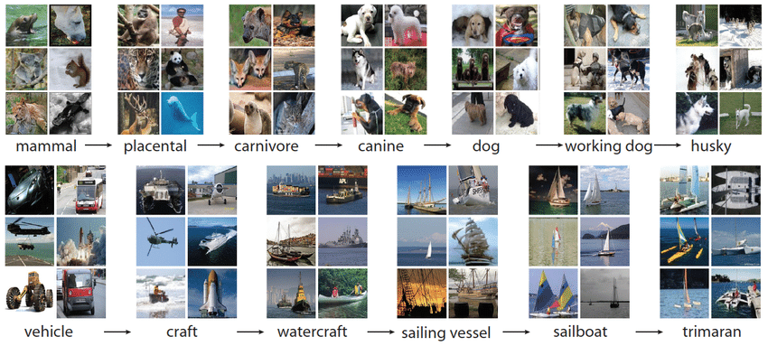
The rise of deep learning is best told through ImageNet, a landmark dataset introduced by Jia Deng, Fei-Fei Li and collaborators in 2009. ImageNet was an enormous collection of labeled images — millions of photographs organized into tens of thousands of categories according to WordNet’s semantic hierarchy.

What made ImageNet transformative was not just its size but that it also established a shared benchmark. A subset of classes became the basis for an annual competition called ILSVRC (ImageNet Large Scale Visual Recognition Challenge), which started in 2010: teams worldwide trained their models on the same images and were scored on the same held-out test set. This created something machine vision had lacked — a common, fair setting where different approaches could be compared directly.

With this benchmark in place, two other forces did the rest:

• GPU computation and deep networks made it practical to learn increasingly effective visual representations directly from raw pixels — no hand-crafted features needed.
• The benchmark itself made differences in performance visible under identical conditions, so an advance like AlexNet (which we examine next) could be seen immediately and unambiguously by the whole research community.

The central lesson is that a full research transition depends on the relationship among data, model, training, hardware and evaluation. ImageNet alone was just data; deep networks alone had existed for years; GPUs alone were video-game chips. The revolution came from combining all of them under one shared measurement standard.

A quick note to keep your timeline straight — these are distinct events that should not be blurred together:

• 2006: deep belief networks helped revive interest in training deeper models (a separate thread).
• 2009: ImageNet itself is published.
• 2010: the ILSVRC competition begins.
• 2012: AlexNet wins by a wide margin and announces deep learning’s arrival — our next section.

A few clarifications will help you reason precisely about ImageNet rather than treating it as a single blurry thing. First, distinguish two different collections that share the name:

• The full ImageNet archive: millions of images across tens of thousands of semantic categories — a general-purpose resource for studying visual recognition and organization.
• The ILSVRC classification task: a specific benchmark built from a subset of 1,000 classes (about 1.2 million labeled training images), used in the annual competition to compare models under identical conditions.

These differ in size and purpose. When people say “AlexNet won ImageNet,” they mean it achieved the best accuracy on this specific 1,000-class benchmark task — a precise claim that should not be inflated into “solved all of computer vision.”

The montage below illustrates what makes ImageNet special: its variety and semantic organization. Images are grouped according to meaning (via WordNet), so the dataset is structured rather than merely big — which helped models learn genuinely useful visual concepts.

Two conceptual points keep your understanding honest:

1. A benchmark defines an evaluation task, not every aspect of intelligence. Scoring well on ImageNet means doing well at its specific protocol (label one central object in a photo). It says nothing directly about captioning scenes, answering questions or driving cars. Benchmarks are valuable precisely because they are narrow and measurable — that clarity is their strength.
2. Success measures the specified protocol. So when the field celebrates an ImageNet result, it is celebrating mastery of a well-defined task under shared rules — which is why benchmarks have been so powerful for driving progress: everyone agrees on what “winning” means.

Finally, keep several milestones distinct in your mind. The 2009 ImageNet publication differs from the 1,000-class ILSVRC task (2010 onward). Later developments — residual networks and attention-based methods like Transformers — continued the same story of representation and optimization but under changing data and evaluation demands. And to avoid a common confusion: word2vec’s CBOW/skip-gram models (word vectors, 2013) are quite different from the 2017 Transformer architecture, even though both concern representing language.

AlexNet, built by Alex Krizhevsky, Ilya Sutskever and Geoffrey Hinton in 2012, is the moment deep learning burst into mainstream attention. At that year’s ILSVRC competition — the shared benchmark described earlier — AlexNet delivered a result dramatically better than everything else on the table, reducing top-5 test error from the runner-up’s 26.2% to 15.3% for the winning entry (about a 42% relative reduction). It was not an incremental improvement; it looked like a different kind of system.

What made AlexNet so effective? Several factors combined:

• A deep convolutional architecture: many layers organized hierarchically to detect features from simple (edges, textures) to complex (faces, objects), building on the Neocognitron/CNN ideas we met earlier.
• Substantial computation, made practical by training on GPUs — an early and influential use of graphics hardware for deep learning at scale.
• Good training choices: ReLU activations (which helped reduce gradient attenuation on their positive side), dropout to reduce overfitting, data augmentation to get more variety from the same images.

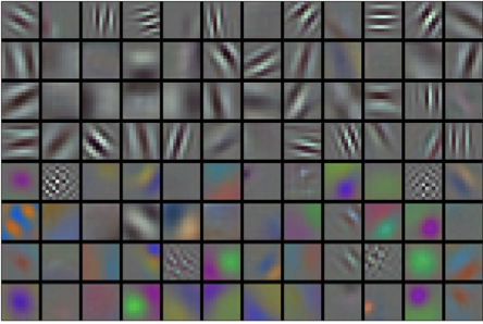
A particularly telling detail is what AlexNet’s learned first-layer filters looked like: they showed recognizable local visual patterns — oriented edges and color blobs — strikingly similar to features that neuroscientists had long associated with early human vision. Yet these were not hand-authored by engineers; they emerged automatically from training on data. This made vivid the connectionist promise: useful representations could be learned, not designed.

The result became prominent precisely because it happened in a shared comparison setting (ILSVRC) — everyone ran under identical conditions, so there was no dispute about who had won or by how much. Benchmarks, as we saw, convert an advance into a visible, verifiable event.

Finally, read AlexNet the right way: its success illustrates the combined effect of architecture, training choices, data and hardware working together — consistent with everything from earlier sections. It does not support a naive slogan like “just add more layers and every model improves automatically.” Adding depth helps only when supported by good training methods, enough data and sufficient compute. AlexNet is best understood as the moment these ingredients reached critical mass.

The final era brings AI into the present day — a burst of progress so visible in everyday life it hardly needs an introduction. But before we look at specific systems, notice that this modern wave actually combines several distinct research strands, each with its own mechanism:

• Learning combined with search. Systems like AlphaGo pair a learned ability to evaluate positions with the older AI idea of searching through possible moves — connecting back directly to the TuroChamp chess algorithm from Part 1, but now supercharged by deep learning.
• Large-scale sequence modeling. The Transformer architecture and its descendants reorganized how machines process language by focusing on what is most relevant (attention), then scaled up enormously. These are the engines behind modern chatbots and text generators.
• Accessible interfaces. Conversational front-ends let non-specialists use powerful models simply by typing — turning research systems into consumer tools that reached hundreds of millions of people almost overnight.

The crucial point is captured in the phrase “their mechanisms remain different.” AlphaGo choosing a Go move, a Transformer predicting the next word, and an image generator producing art all get lumped together under “modern AI,” but they work by genuinely different principles. It would be sloppy — and it will confuse you later — to treat them as one homogeneous technology just because they arrived in the same era of public excitement.

As we go through AlphaGo, Transformers/large language models and ChatGPT-style interfaces over the next few sections, keep asking: what exactly does this system compute, and how? The ability to separate these mechanisms is what separates real understanding from headline-following.

The modern era weaves together several independent strands of research into what the public now calls “AI.” It helps to name each strand so you never confuse them:

• AlphaGo: a system that plays Go at superhuman level by combining learned evaluations (a neural network estimates how good a position is) with search (exploring promising move sequences). It connects learning and search — two themes running through all of AI history.
• The Transformer: an architecture that reorganized sequence processing around the idea of attention, letting each part of a sentence focus on whichever other parts matter most. This became the basis for large language models, which scale up this architecture and objective (predicting the next word) to enormous sizes.
• Conversational interfaces: front-ends that wrap these powerful models in an easy-to-use chat format, making capabilities that were once research curiosities accessible to anyone with a browser or phone.

The single most important thing is to keep the milestones distinct. The early AlphaGo results (beating European champion Fan Hui in 2015), the famous 2016 match against Lee Sedol, and the separate 2017 Transformer paper are three different events from different research programs — not one happening. Blurring them together produces a muddled story.

Likewise, this era is best understood as bringing several strands together, not providing one single explanation for all progress. Different systems solve different problems with different mechanisms.

A note on terminology, because “generative AI” gets used loosely: generative models are those that produce new content. The family includes not only text generators but also generative adversarial networks (GANs, 2014) — where two networks compete to generate realistic images — and diffusion models such as DDPM (2020), which learn by progressively removing noise from images. Crucially, AlphaGo is a game-playing system that evaluates positions; it does not generate language or pictures, so despite being famous and “modern,” it is not itself a generative model.

Two of the most celebrated milestones of modern AI — AlphaGo and the Transformer — are easy to lump together as “recent breakthroughs,” but understanding them properly means seeing how different they really are. Let’s take each in turn.

• AlphaGo: learning + search for game play. Go has a famously enormous space of possible continuations — far too many for any machine (or person) to explore exhaustively, even with unlimited time. AlphaGo tackled this the same way good chess programs always have, by combining two ideas: search through promising move sequences, and learning, specifically a neural network trained to evaluate how good any position is without needing to look ahead all the way. Learning guided which branches of search were worth exploring; search verified them deeply. Their cooperation proved enough to beat top human players.
• The Transformer: attention for sequences. Published in 2017 as a separate contribution, the Transformer reorganized how machines process sequential data (text). Instead of reading a sentence strictly word by word, it uses an attention mechanism that lets every position weigh how relevant all other positions are — so “bank” can look back at context to decide whether it means river bank or money bank. This attention-based architecture proved extremely effective for sequence processing and generation, becoming the backbone of modern language models.

The contrast matters because their demonstrated tasks and mechanisms differ: AlphaGo chooses game actions through search over a board; the Transformer organizes how to process and generate sequences by attending across positions. Both are landmarks — but they are different kinds of systems solving different problems, which is exactly why you should not treat “modern AI” as one undifferentiated thing.

Finally, keep the timeline precise. AlphaGo defeated European champion Fan Hui in 2015 and world-class player Lee Sedol in 2016. The trailer shown with this section concerns that famous 2016 Lee Sedol match. The Transformer paper, “Attention Is All You Need,” was published in 2017 — after and separately from these matches.

GPT-3, introduced by OpenAI in its 2020 paper, is the clearest example of how Transformer language models work — and it helps to demystify what “generative AI” actually does under the hood.

Technically, GPT-3 is a decoder-only Transformer language model. The key phrase here is next-token prediction: given everything that has been written so far (the preceding context), the model produces a probability distribution over which token — roughly speaking, which word or piece of a word — should come next. It does not search its memory for a prewritten answer to your question; it computes, from scratch, what token is most likely to follow in this particular context.

The diagram for this section illustrates that operation: you feed in context on the left, and out comes a distribution over possible next tokens. Now here is the remarkable part — repeating this single step generates an entire continuation. You predict one token, append it to the context, predict the next from there, and so on until the text stops. A whole essay or chat reply emerges from looping a very simple “predict what comes next” operation many times.

That mechanism explains both GPT-3’s impressive fluency and its limitations:

• The model is trained only to produce plausible continuations of text. Fluency does not equal correctness — because the training objective rewards “what usually follows,” a model can confidently generate plausible-sounding statements that are false.
• The output is shaped by both its learned patterns and whatever information you supply in context. Give it accurate background or clear instructions, and the result improves; give it nothing (or misleading context), and it will simply continue from what little it has.

A few precise facts to keep straight: GPT-3’s largest configuration had 175 billion parameters — an enormous number of internal weights learned during training. And its “few-shot” behavior is a subtle point: you can give examples inside the prompt (say, three English-to-French translations) and it will follow that pattern for the next answer — but this happens entirely through context, with no gradient updates to the model’s weights. It adapts at inference time by reading your prompt, not by retraining.

The “bitter lesson”, articulated by AI researcher Richard Sutton in a widely read 2019 essay, is not a technical theorem but an argument about research strategy — and one of the most influential pieces of writing on how to think about progress in AI.

Sutton’s observation comes from looking back at decades of history: again and again, researchers tried to build intelligence by hand-crafting knowledge into systems (hand-written rules, manually designed features, carefully engineered representations). For a while these approaches look very smart. But over the long run, Sutton argues, the methods that ultimately win are the general ones — above all learning and search — because they can exploit one resource that keeps growing without bound: computation.

• Learning: instead of telling the machine the rules, we give it lots of data and let an algorithm discover patterns. As computers get faster and datasets larger, learned models keep getting better.
• Search: rather than encoding every possible situation, provide a general search procedure that can explore — again benefiting directly from more computation to look further or deeper.

The lesson is called “bitter” because it suggests that much painstaking human cleverness spent on hand-authoring intelligence ultimately matters less than we would like. The curves you see in the lecture are conceptual illustrations of this idea — not measured historical data points, but a schematic picture of how general methods overtake specialized ones as compute grows.

It is essential to interpret Sutton’s argument precisely and avoid overcorrecting:

• His essay is a perspective on strategy, urging researchers where to invest effort — not a mathematical proof that algorithms, representations or domain knowledge never matter.
• Indeed, even “general” methods still require careful design of their architecture and objective. The point is comparative: approaches whose capabilities scale with available resources tend to outrun those bounded by how much structure humans can hand-author in advance.

The bitter lesson invites you to weigh two styles throughout AI history — scaling-friendly general methods versus knowledge-rich specialized designs — and notice which has more often won as computation grew. It is a lens, not a law, but one that helps explain the trajectory from 1950s perceptrons all the way to today’s massive learned models.

The launch of ChatGPT in late 2022 marked AI’s arrival as a mainstream consumer technology almost overnight. But it is important to understand precisely what ChatGPT was: not an entirely new kind of model, but a conversational interface wrapped around a language model that had been further adapted for interaction.

The story has two distinct stages, and keeping them apart clarifies how such systems are built:

1. Pretrained next-token modeling. First, a large Transformer (in the GPT lineage) is trained on vast amounts of text to predict what comes next — learning broad patterns of language. At this stage it can generate fluent continuations but does not yet behave like a helpful assistant that follows instructions and answers questions directly.
2. Adaptation for interaction. The base model is then further refined so it responds usefully in dialogue, notably by learning from human feedback. Human annotators rate or rank the model’s responses; those preferences are used to tune behavior toward being helpful and following the user’s intent. This second stage — instruction-following aligned with what people find good — is what turns a raw language generator into something that feels like an assistant.

The example exchange shown in this section demonstrates the accessibility that made ChatGPT revolutionary: anyone can type a plain-language request — “explain Bayes’ theorem to me” or “summarize this text” — and receive an answer directly in dialogue, with no programming skill required. This is a genuine shift from AI as research tooling to AI usable by everyone.

Two cautions keep your understanding accurate:

• The description here concerns the launch period. Later versions introduced many further changes; treat this section as explaining what made the milestone famous, not as a complete specification of every version that followed.
• The displayed conversation is an invented teaching illustration, created to show how such exchanges look — it is not a verified transcript captured from the actual 2022 release. And remember, from our GPT-3 discussion: even a well-aligned chatbot can produce fluent but incorrect content; fluency never guarantees truth.

With ChatGPT, generative AI moved from research papers into everyday life — completing the arc this lecture has traced from probability and neurons to systems billions of people now use.

On 15 September 2026, TypeSafe announced Jev in early access, using the name System One models for its approach. The aim is fast, bounded judgments that a program can consume directly. The name draws on the idea of fast human judgments; it is a design analogy. This is a recent provider announcement, rather than a settled historical verdict. Source: TypeSafe’s announcement.

From a message to a usable decision

Imagine a customer writes, “I was charged twice.” A program supplies the message and asks which team should handle it, limiting the answers to Billing, Technical support or Other. Our invented classroom output is Billing, with probabilities 0.90, 0.03 and 0.07 respectively. Code can then route the request or ask for review. These numbers illustrate the interface; they are not measured model results.

The documentation describes questions for selecting an option, assigning a rubric score or assessing a statement. Several questions can be evaluated in parallel against the same information. Jev does not generate free-form text. Language models can also return structured answers; Jev emphasizes a model designed specifically for decisions. Source: TypeSafe’s introduction.

What makes a probability useful?

TypeSafe calls its training approach Reinforcement Learning for Calibrated Decisions (RLCD). Calibration means that, across many predictions assigned 80% probability, the predicted outcome should occur about 80% of the time. It is a property assessed across predictions, not certainty about an individual answer. This reconnects modern automation to the course’s earlier discussion of uncertainty. Source: TypeSafe’s AI primer.

For Choice and Score, the API also supplies a confidence measure derived from the distribution. Software can use uncertainty to defer a decision, gather information or request human review. Thresholds should be tested for the intended task. Source: TypeSafe’s confidence documentation.

Keep structure and correctness separate

A permitted answer can still be wrong. Returning Billing respects the category list, but does not prove Billing is the right destination. Interpret the announcement’s no-hallucination claim narrowly: guaranteed output structure does not guarantee factual accuracy. Its speed comparisons are provider-reported, and its workflow evaluations use other models’ probabilities as references. They do not establish universal superiority or correctness. The useful historical connection is the combination of learned judgments, explicit software constraints and uncertainty.

Open the Jev example slide → · Open the calibration slide →

Now that you have followed AI from its statistical birth all the way to modern generative models, step back and notice the deep pattern running through this entire history: AI repeatedly combines established ideas with new opportunities. Very few genuine breakthroughs were invented from nothing; most arrived when older concepts — probability, search, feedback, neurons, rules — met fresh resources in data, computation and implementation.

Five threads keep interacting across every era:

• Inference: reasoning from evidence (Bayes’ theorem onward).
• Search: systematically exploring possibilities toward a goal (from TuroChamp to AlphaGo).
• Feedback: regulating behavior by observing and correcting (cybernetics, then reinforcement learning).
• Symbolic reasoning: manipulating explicit rules and logic (Logic Theorist, expert systems).
• Learned representations: letting models discover their own internal structure from data (perceptrons to deep networks).

These strands were not a linear sequence where each replaced the last. They coexisted and combined — AlphaGo literally fuses learning with search; modern language models combine learned representations with attention-based processing.

The history also delivers two complementary lessons:

1. Periods of disappointment caution against over-generalizing from restricted demonstrations. Every winter began when someone treated a narrow success as proof that general intelligence was solved. Stay humble about what any single result really shows.
2. Sustained progress demonstrates the value of reusable principles. Ideas like search and learning kept paying off across decades precisely because they are general, not tied to one gimmick or task.

These recurring, transferable ideas — rather than any single famous program — are what make AI a coherent field. The next chapter examines one of the most fundamental reusable principles in detail: systematically searching through possible actions, while tracking costs, goals and unfinished alternatives. That is the subject of search algorithms.

You have now seen the full arc of AI history — two centuries of foundations compressed into a story of cycles: excitement, disappointment and renewal on stronger footing. Before moving to search algorithms in the next lecture, check your grasp with three core takeaways:

• Explain why AI progress includes setbacks as well as breakthroughs. Each “winter” followed inflated expectations that outran what the technology could deliver — e.g., Minsky and Papert showing single-layer perceptrons cannot solve XOR, or commercial hype cooling in the late 1980s. Yet each downturn was followed by renewal on firmer foundations (better data, compute, training). Progress is not a smooth line but a staircase with real dips.
• Distinguish rule-based expertise from learning from data. Expert systems encoded human knowledge explicitly as if–then rules (MYCIN’s medical rules), requiring painstaking acquisition and maintenance. Learning-from-data approaches instead adjust parameters automatically — perceptrons fixing errors, backpropagation tuning weights from examples. One hands the machine the answer; the other lets it discover patterns.
• Describe how data, computation and learning contribute to modern AI. Modern systems like ImageNet-era deep networks succeed when large datasets meet fast GPU compute and effective training algorithms — each reinforcing the others (the virtuous cycle). AlphaGo pairs learned evaluation with search; GPT-3 scales next-token prediction over billions of parameters. None of these ingredients alone explains the result.

Now choose one of these three ideas and explain it in your own words using a concrete example from this part — perhaps XOR and the perceptron limit, MYCIN versus backpropagation, or how ImageNet plus GPUs ignited deep learning. Teaching it back is the surest way to confirm you have truly absorbed Part 2.