Regression · Part 1
Fit numerical predictions and compare simple and flexible models using both training and held-out evidence.
From observations to a fitted prediction rule
Regression predicts a numerical response from one or more inputs. Begin with the observed pairs, specify a candidate mean function, choose its coefficients by least squares and evaluate its predictions. Then allow polynomial features to represent curvature.
Part 1 follows linear regression, training, model evaluation and polynomial regression. Part 2 continues with bias–variance, accuracy of estimates, multiple regression and assumptions. The notation and examples below make each step explicit.
Inspect 25 fertilizer and yield observations
Inspect the 25 paired fertilizer and yield observations before choosing a family. Look for direction, curvature, unusual points and changing spread. Every dot is one input–response pair; selecting its number reveals its coordinates. The illustrative scales have no specified physical units.
The scatter suggests that a line may summarize the trend. It does not establish that fertilizer causes the response, and it does not determine how well predictions will transfer to new cases. Use the plot to formulate a candidate model, then evaluate it.
Try it: Each dot is one trial: input x = fertilizer, response y = yield. Select a point, zoom or pan to inspect the trend.

Static preview. Open handout.html to use the interactive example.
Start with a line as an approximate prediction rule
Simple linear regression predicts a numerical response using one input. A dataset contains n recorded pairs (xᵢ, yᵢ), where i identifies a trial. In the fertilizer example, xᵢ is the recorded fertilizer level and yᵢ is the measured yield. The demonstration uses illustrative scales; physical units are unspecified.
We choose a straight-line family f(x) = β₀ + β₁x. Different intercepts β₀ and slopes β₁ give different candidate lines. Their values are unknown and will be estimated from training observations later. Evaluating a candidate at xᵢ gives f(xᵢ), its proposed response for that input.
The statement yᵢ ≈ f(xᵢ) expresses an approximate relationship. It does not claim that every observed response is exactly the line’s value, nor that the difference is merely a rounding error. The next example makes that difference concrete.
n = number of training trials
f = prediction function.≈ means “approximately equal”: the observations need not lie exactly on the line.
The same input can give different observed responses
For this worked example only, suppose the true mean relationship is f(x) = 1 + 3x. The intercept is 1: at x = 0 the mean response is 1. The slope is 3: moving one unit along the input axis raises the mean response by 3 units. Its units are response units per input unit.
A slope of 3 compares the mean responses: f(2) = 7 and f(3) = 10. It does not compare a particular pair of measured yields. For example, a measured response of 8 at x = 2 and 9 at x = 3 differs by only 1 because the individual deviations from the means are +1 and −1.
At x = 2 the mean response is 7, but individual observations can be 6 or 8. The two cases have the same recorded input and different outcomes. Variation from unrecorded factors, natural randomness or measurement noise can produce such differences.
The diagram assumes a known mean line to explain the idea. With real data we do not know that true line; estimating it is the training problem. Also check whether x = 0 is meaningful before giving the intercept a practical interpretation.
At x = 0, the line’s mean response is 1. This is where the line meets the vertical axis.
At x = 2, the mean is 7; at x = 3, it is 10: an increase of 3. Actual responses can lie above or below those means, so two measured yields need not differ by 3.

Make the approximation explicit: add a random error
The approximate relation yᵢ ≈ f(xᵢ) becomes the observation model yᵢ = f(xᵢ) + εᵢ = β₀ + β₁xᵢ + εᵢ. Here εᵢ, pronounced epsilon i, is the random deviation of response i from the systematic line. Adding the error term accounts for the discrepancy; it does not eliminate it or imply perfect prediction.
The term is broader than a measurement mistake. It may include natural variation, unrecorded influences and measurement noise in the response. It is a response-side deviation, not simply an error “associated with measuring the input xᵢ”. In the worked example, f(2) = 7: a response of 8 has ε = +1, while a response of 6 has ε = −1.
To interpret the line as a mean response, assume E[ε | X = x] = 0 for each x. E means an average or expected value and | reads “given”. Under this assumption E[Y | X = x] = f(x): repeated observations at the same input average to the line, even though individual observations vary. The error term introduces a probabilistic model, which will later support uncertainty calculations.
In real data the true coefficients and errors are unknown. After fitting an estimated line, we can calculate a residual rᵢ = yᵢ − , where the hat marks a fitted prediction. A residual is therefore observable after fitting; it is an approximation to, not the definition of, the unobserved random error εᵢ. The forthcoming residual example develops this distinction.
y = 6 gives ε = −1.Assume the errors average to zero at each x. Then f(x) is the mean response at that input.
Optional self-check
A toy model predicts yield = 2 + 3x, where x is fertilizer in kilograms. We express the same input as z = 1000x grams. Which model gives exactly the same predictions?
- Yield = 2000 + 3000z.
- Yield = 2 + 3000z.
- Yield = 0.002 + 3z.
- Yield = 2 + 0.003z.
A residual measures one prediction’s vertical miss
For a current candidate line, write its prediction at input xᵢ as . The residual rᵢ = yᵢ − compares the recorded response with that prediction at the same input. If the response is 8 and the prediction is 7, the residual is +1. A prediction of 9 for the same response would instead give −1.
The sign tells us which side of the line the observation occupies: positive means underprediction, negative means overprediction, and zero means exact agreement on that case. This is a vertical response difference, not the shortest distance to the line.
We can compute these discrepancies for a candidate line or a fitted line. The random error εᵢ instead describes deviation from the unknown true mean relationship. It is not directly observed when that relationship is unknown.
yᵢ = observed response
= the current line’s prediction.A residual is a vertical response difference at the same input xᵢ, not a perpendicular distance.
We need one score to compare candidate lines
There are infinitely many possible intercept–slope pairs. Visual inspection may suggest a plausible line, but we need a common numerical criterion to decide which candidate is better. Comparing one point at a time is insufficient because changing the line generally helps some predictions and hurts others.
Adding signed residuals fails: both (+2, −2) and (+1, −1) add to zero even though the second candidate is closer on both cases. Ordinary least squares uses the residual sum of squares, abbreviated RSS: square every residual and add the results. These candidates score 8 and 2, respectively.
Squaring makes each contribution nonnegative and penalizes large misses more strongly. Absolute deviations would be another possible objective; RSS is the particular criterion used by ordinary least squares. Comparing RSS values is meaningful here because both candidates are scored on the same observations.
Least squares adds the squared vertical gaps
For the current coefficient pair β = (β₀, β₁)ᵀ, calculate the prediction = β₀ + β₁xᵢ at each of the n training inputs. Subtract it from yᵢ, square that residual and add the n contributions. This is RSS(β), a score for that candidate line.
The hat on identifies a predicted response. The coefficients β are still candidate values at this point; the fitted optimum will be written . Squaring prevents cancellation and emphasizes larger misses. RSS has squared response units and is a sum, not a variance. A small training RSS alone does not establish good predictions on new cases.
n = training count. = prediction
rᵢ = observed minus predicted
RSS = residual sum of squares.
Self-check
Two observed responses are 2 and 4; a line predicts 3 for both. Residual = observed minus predicted. What does the zero sum of residuals tell us?
- The fit is exact because its positive and negative errors sum to zero.
- The residual sum is zero, so RSS must also be zero.
- The residuals cancel, but RSS = 2: neither prediction is exact.
- The model overpredicts both cases, with RSS = 4.
Training means choosing the coefficients with the smallest RSS
Ordinary least squares (OLS) is a fitting rule: choose the coefficients that make the sum of squared prediction errors (RSS) as small as possible.
Ordinary least squares, abbreviated OLS, is an optimization rule: among all real intercept–slope pairs, choose a pair minimizing the training RSS. The operator arg min returns the coefficient vector that achieves the minimum. In contrast, min returns the minimum value of the objective.
“Least squares” means minimizing the sum of squared vertical response errors. “Ordinary” distinguishes the equal-weight version: every squared residual enters with coefficient 1. Weighted least squares would give different observations different weights. The line family is specified first, then OLS selects its coefficients.
This operation is called parameter estimation in statistics and model fitting or training in machine learning. It defines how to choose a hypothesis from the family. It does not specify how the data were sampled or guarantee that the chosen family describes the true relationship.
= fitted coefficient pair.ℝ² = all pairs of real numbers
OLS = ordinary least squares.
Move the line and watch the residuals change
Change the intercept and slope to move the candidate line. At each fixed input, the vertical segment joins the observation to the line. A point above the line has a positive residual; a point below has a negative residual. These are vertical, not perpendicular, distances.
The controls recompute RSS for the current candidate. Fit OLS uses the analytic optimum on the same 25 observations. Compare its error with your manual choices, then move the line again to see why improving one point can worsen others. The optimum minimizes the aggregate squared error.
Try it: β₀ moves the line up or down; β₁ changes its slope. Watch the residuals, then press Fit OLS to minimize RSS.

Static preview. Open handout.html to use the interactive example.
Where do the slope and intercept formulas come from?
They solve the OLS problem: minimize RSS. Differentiate RSS with respect to β₀ and β₁, set both derivatives to zero, then solve the two equations.
The OLS slope divides the centered input–response cross-product by the total centered input spread. Subtracting and centers each variable. The means are = (1/n)∑ᵢxᵢ and = (1/n)∑ᵢyᵢ, with sums over all n training observations.
Once the slope is fitted, choose the intercept so that the line passes through (, ). These formulas require Sxx = ∑ᵢ(xᵢ − )² > 0. For example, input values 0, 1, 2 and responses 1, 3, 5 have means 1 and 3, slope 2 and intercept 1. If all inputs are equal, slope and intercept cannot be identified separately.
Derivation from the RSS objective
A partial derivative, written ∂, measures how RSS changes when one coefficient changes while the other stays fixed. At a minimum, both coefficient directions have zero derivative.
The first equation says that the residuals sum to zero. Rearrange it to get β₀ = − β₁. Substitute this into the second equation and collect the centered terms:
Divide by the sum of squared centered inputs to obtain the fitted slope shown below. Substitute that slope into the intercept equation to obtain the fitted intercept. Hats mark the resulting fitted estimates.
RSS is a convex quadratic function, so these equations identify a global minimum. The solution is unique when the inputs are not all equal, making the denominator positive. Computing OLS does not require normally distributed errors.
= (1/n)∑yᵢ: training sample means. = fitted slope
= fitted intercept
all sums use i = 1,…,n.
When do the data determine one best-fitting line?
Trials use x = 0, 1 and 2.
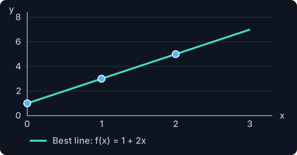
The best slope is 2 and the intercept is 1.
Tilting or shifting this line increases RSS.
All three trials use x = 2. Their responses are 4, 5 and 6.
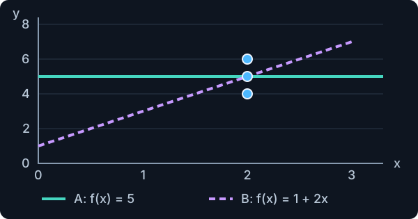
Both lines predict 5 at x = 2 and have RSS = 2.
These trials cannot tell us which slope to choose.
A unique best-fitting line means that exactly one intercept–slope pair minimizes training RSS. For simple linear regression with an intercept, this happens when the training inputs include at least two different values.
In the left example, the observations are (0,1), (1,3) and (2,5). The line f(x) = 1 + 2x passes through all three points and has RSS = 0. Any different line must miss at least one point and therefore has a larger RSS.
In the right example, all trials use the same input x = 2, but their measured responses are 4, 5 and 6. For example, each trial might use exactly the same fertilizer dose while the measured yield varies. The best prediction at that dose is the response mean, 5. Both f(x) = 5 and f(x) = 1 + 2x predict 5 there, so both have RSS = (4−5)² + (5−5)² + (6−5)² = 2. In fact, every line through (2,5) gives this same minimum training error. Those lines can predict very differently at other inputs, where we have no observations.
What did “every x equals c” mean?
It means x₁ = x₂ = … = xₙ = c: every observation has the same input value. The letter c merely stands for that common value. In the example, c = 2. The responses y₁,…,yₙ need not be equal. At x = 2, a line predicts β₀ + 2β₁, so many intercept–slope pairs give the same best value, 5.
More generally, when every input equals c, the best coefficients need only satisfy , where the bar denotes the training response mean. This is one equation for two coefficients, leaving many possible lines.
What is full column rank?
A design matrix stores the model’s input features in columns. Full column rank means that no column can be obtained by combining the other columns. Each column therefore adds independent information for estimating coefficients. For a straight line, the two columns contain a constant 1 and the input x. If every x is 2, the input column is twice the column of ones. The two columns are redundant, so the coefficients cannot be determined separately. If the inputs vary, those two columns are independent. The matrix notation is developed later in this lecture.
Why was convexity mentioned?
Convexity describes the RSS objective as a function of its coefficients. It rules out a local minimum that is worse than the global minimum, but it still allows a flat set of equally good minima. In the same-input example, changing slope and intercept together can leave every training prediction unchanged. The elementary condition we need here is simply that the inputs vary.
Compare a candidate line with the exact OLS fit
Self-check
On the same three training cases, line A has residuals (0, 0, 3), and line B has (2, 2, 0). Which line does ordinary least squares prefer?
- Line B: its RSS is 8, compared with 9 for line A.
- Line A: it predicts two of the three cases exactly.
- Line A: its signed residual sum is smaller.
- They tie because both have a residual equal to zero.
The purpose of this example is to show what fitting changes. We keep the same 25 training observations and compare two choices of intercept and slope.
A candidate line is simply a proposed prediction rule. The starting guess here is f(x) = 2 + 2x: intercept 2 and slope 2. We chose these simple coefficients for illustration, without minimizing RSS. The candidate has RSS ≈ 9.6666.
Press Show OLS best fit. The green line is calculated from these 25 observations using the least-squares formulas: fitted intercept ≈ 2.1339 and fitted slope ≈ 2.8261. Its RSS is ≈ 0.3106, much lower than the starting guess. The purple dashed line remains visible so that the comparison is direct.
The observations do not change. OLS changes the coefficients to minimize the sum of squared vertical prediction errors. This demonstrates the difference between proposing a line and fitting one. The fitted line need not pass through every dot because the observations are noisy.
The OLS best fit is calculated directly from the displayed observations. A starting guess could happen to be close to that solution. Here we deliberately choose a more visibly different guess to make the purpose of fitting clear.
Try it: A candidate is a proposed line. We deliberately start with f(x) = 2 + 2x. Press Show OLS best fit to see how minimizing RSS improves this guess.

Static preview: the starting guess and OLS best fit are both shown. Open handout.html to reveal or hide the fitted line.
Model evaluation: what does a good score tell us?
Evaluating a model often means using one or more metrics to estimate its quality with respect to particular aspects of a task. Examples include its predictive ability and its robustness to noise. A metric is a numerical summary of one aspect of performance, so no single score answers every question about a model.
Although calculating a score can seem straightforward, evaluation hides pitfalls. The interpretation depends on the selected metric, the observations on which it is calculated and the way those observations were used during fitting or model selection. Interpreting the results takes care and experience.
Here we focus on how well the model explains the observed data and how well it generalizes to new instances. We begin with two popular evaluation metrics for linear regression: residual standard error (RSE) and the coefficient of determination (R²). RSE estimates the remaining error scale from training residuals, in response units. R² compares the model’s squared error with a mean-response baseline.
These measures first help us interpret the fit to observed data. A good training score alone does not establish generalization. Later, we keep the model fixed and evaluate predictions on held-out observations, which were not used to fit its coefficients, using root mean squared error (RMSE). Part 2 addresses uncertainty in the estimated coefficients.
Training performance: how closely does the line fit?
Training performance describes how well a fitted model explains the observations used to estimate its coefficients. Residual standard error (RSE) summarizes the remaining vertical prediction errors. On the same observations, using the same number of fitted coefficients, a lower RSE means the fitted predictions are closer to the recorded responses.
Fitting the intercept and slope to these same observations makes their residuals look optimistic. The n − 2 correction accounts for those two estimated coefficients. A two-point example helps show why dividing by n is not enough.
For a line with an intercept, we estimate two coefficients from n training cases, leaving n − 2 residual degrees of freedom. Under a correctly specified mean, independent equal-variance errors and nonconstant inputs, RSE² = RSS/(n − 2) estimates the common error variance. RSE is the square root, so it estimates an error standard deviation and has the response’s units. For example, RSE = 2 kg describes an estimated error standard deviation of 2 kg.
RSE is nonnegative and has no fixed upper bound. It is an absolute measure: its numerical value changes when response units change, and whether 2 kg is acceptable depends on the task and the response scale. A relative comparison with a simple prediction rule helps us judge the model’s improvement.
For a full-rank model with q independent fitted coefficients, replace n − 2 by n − q. A degree-p polynomial has q = p + 1. Positive residual degrees of freedom are required. RSE² is an unbiased variance estimator under the stated assumptions, while its square root is not exactly unbiased.
n = number of training observations
i = observation index, from 1 to n.yᵢ = observed response
= fitted line’s prediction
Require n > 2, varying inputs and the stated linear-model assumptions.
Intuition for the n − 2 correction
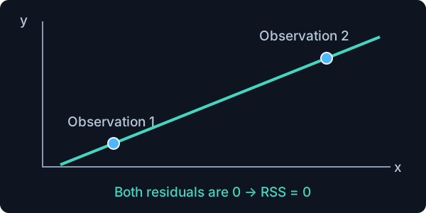
A line can pass through both points exactly.
RSS = 0 does not prove that the measurements were noise-free.
Start with n observations.
Estimate 2 numbers: the line’s height (intercept) and tilt (slope).
That leaves n − 2 independent pieces of information in the residuals to estimate the noise.
Example: 10 observations → 10 − 2 = 8 residual degrees of freedom.
The line is chosen to reduce errors on the same observations that we later use to measure its residual scatter. Moving and tilting the line can partly follow accidental measurement noise. The resulting training residuals are therefore smaller than they would be if the true mean line had been known in advance. Simply dividing their squared sum by n would underestimate the noise variance.
A straight line has two freely estimated coefficients: its height (intercept) and tilt (slope). Estimating them uses two independent pieces of information. Under the stated linear-model assumptions, n − 2 independent pieces of information remain in the residuals for estimating the error variance. These are called residual degrees of freedom.
The two-point thought experiment makes the need for a correction visible. Any two observations at different inputs have a line passing through them exactly. Both residuals are zero, so RSS = 0 even if the measurements were noisy. With n = 2, n − 2 = 0: those residuals cannot estimate the noise scale. This is why the RSE formula requires more than two observations.
With 10 observations, fitting the two coefficients leaves 8 residual degrees of freedom. All 10 observations are still used in both fitting and the residual sum. We do not discard two observations. Dividing RSS by 8 rather than 10 corrects the noise-variance estimate for the two coefficients fitted from those data, then taking the square root gives RSE.
More precisely, fitting a line with an intercept makes the residuals satisfy two relationships: their sum is zero, and their input-weighted sum is zero. These two constraints explain why the residuals provide n − 2, rather than n, independent directions of variation. Under the linear-model assumptions, RSS/(n − 2) is an unbiased estimate of error variance. RSE is its square root and is not exactly unbiased.
From RSE to R²: why use a relative measure?
The main difficulty in using residual standard error (RSE) is that it is an absolute measure in the response’s units. Its possible values are nonnegative, with no fixed upper bound. Therefore, a number such as RSE = 2 does not, by itself, tell us whether a model is good: the interpretation depends on the units, the response scale and the task.
For example, an error scale of 2 kg is the same as 2000 g. Changing units changes the numerical RSE without changing the predictions’ quality. Similarly, an error of 2 kg may be acceptable in one application and large in another.
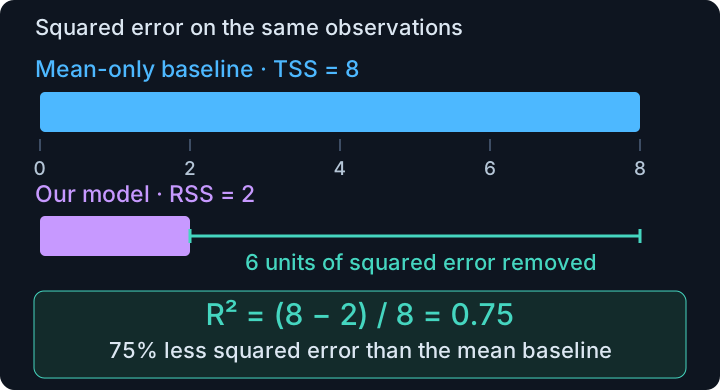
To add context, use a relative measure: the R² statistic, also called the coefficient of determination. It compares the model’s sum of squared errors with the error of a mean-only baseline that always predicts the response average. R² expresses the improvement relative to that reference and is unit-free. Changing response units scales both squared-error totals together, so their ratio stays the same.
The next slide defines the baseline total sum of squares, TSS, gives the equivalent R² formulas and explains how to interpret the score. A relative measure still needs task-specific interpretation.
In the diagram, the mean-only baseline has TSS = 8 and the candidate model has RSS = 2, both on the same observations. The model removes 8 − 2 = 6 units of squared error. Relative to the baseline, that is 6/8 = 0.75, so R² = 0.75. This is a 75% reduction in squared error, rather than a percentage of individually correct predictions.
One possible toy example has responses (2, 4, 6). The mean-only predictions (4, 4, 4) give TSS = 8, while candidate predictions (3, 4, 5) give RSS = 2. These predictions illustrate the score and are not asserted to be the OLS optimum on these three points.
R²: compare the model with a mean-only baseline
To put the absolute RSE scale in context, compare the fitted model with a mean-only baseline, sometimes called a dummy model. It always predicts the training response mean, regardless of input. For a straight line, this means that the intercept is the response mean and the slope is zero. In symbols, the intercept is and the slope is β₁ = 0.
For toy training responses (2, 4, 6), the mean is 4. The baseline therefore predicts (4, 4, 4), with intercept 4 and slope 0. Its squared error is (2−4)² + (4−4)² + (6−4)² = 8. This baseline error is the total sum of squares, TSS. It measures the total squared spread of the responses around their mean.
Suppose a candidate model predicts (3, 4, 5) on the same cases. Its RSS is 1 + 0 + 1 = 2. The ratio RSS/TSS = 2/8 is the fraction of the baseline squared error still left by the model. Subtracting this fraction from 1 gives the relative improvement measured by R². These illustrative candidate predictions are not claimed to be the OLS optimum on these three points.
The coefficient of determination, R², converts the comparison into a relative score. The quantity TSS − RSS is the reduction in squared error compared with always predicting the response mean. Dividing by TSS expresses that reduction relative to the baseline. Equivalently, R² = 1 − RSS/TSS: one minus the fraction of baseline squared error remaining.
The expanded formula uses the same observations in both sums. The numerator adds squared differences between recorded responses and model predictions. The denominator adds squared differences between recorded responses and their mean. For training data, the mean is the training response mean.
With RSS = 2 and TSS = 8, R² = 0.75: a 75% reduction in squared error relative to the mean-only baseline. This is not a claim that 75% of individual predictions are correct. The ratio requires TSS > 0. If every response is identical, TSS = 0 and this raw definition is undefined.
For TSS > 0, the possible range is −∞ < R² ≤ 1. R² = 1 means RSS = 0, so the predictions match all observed responses on that set. R² = 0 means RSS = TSS, so the model and mean-only baseline have the same squared error. R² < 0 means RSS > TSS, so the model performs worse than that baseline.
OLS fitted on its own training data with an intercept cannot have more squared error than its available mean-only candidate. Its training R² is therefore between 0 and 1. On held-out or test data, the model can do worse than the evaluated set’s mean baseline, giving a negative R². This can be a valid generalization result and does not by itself establish that fitting was implemented incorrectly.
There is no universal R² threshold that makes a model good. Useful values depend on the task, measurement noise and field of study. R² is sensitive to outliers: observations far from the overall pattern can strongly influence the sums of squares. Inspect the plots and the application context along with the score. A high training R² alone does not establish generalization or causation.
= model prediction, = response mean
n = number of cases, i = case index.No universal “good” threshold: it depends on the task and field.
Outliers (points far from the pattern) can change the score.
Example: RSS = 2, TSS = 8 → R² = 0.75.
Self-check
On held-out data, a model has RSS = 50 and the mean-response baseline has TSS = 40. Using R² = 1 − RSS/TSS, which interpretation is correct?
- R² = −0.25: the model is worse than that baseline on these data.
- R² = 0.25: the model explains one quarter of the variation.
- A negative value proves that the regression code is incorrect.
- R² is undefined whenever RSS is greater than TSS.
Good training fit does not guarantee good prediction
Training performance alone is not sufficient to evaluate a model’s usefulness. A line can agree well with the observations that determined its coefficients and still predict new cases poorly. Keep observations separate from fitting to assess this generalization.
Training estimates coefficients and any learned preprocessing. Validation compares choices such as polynomial degree. The final test set assesses the selected procedure after these choices are fixed. Repeatedly selecting the best test result turns the test set into development data.
For test RMSE, is the number of test cases. These cases did not fit the fixed model, so there is no subtraction of fitted coefficients from that count. Use later dates or disjoint groups when those match the intended future prediction task.
Test performance: root mean squared error (RMSE)
We use n for the training-set size and for the test-set size. The subscript names the dataset being counted. These counts can differ. The test responses did not estimate the two fitted coefficients, so test RMSE averages over the test-case count without subtracting 2.
Test performance describes how well a fixed, selected model predicts responses on cases not used to fit its coefficients or choose its hyperparameters. In this section we use root mean squared error (RMSE) as the test-performance metric. is the number of test cases, each observed response is compared with its fixed model prediction, and no fitting is performed using these responses.
Square each test prediction error, take the mean of those squared errors over the test cases, then take the square root. The result has the response’s units, making it easier to interpret on the original scale. Lower test RMSE means smaller squared prediction errors on that test set.
For a separate toy test set, observed responses are (3, 5, 7) and model predictions are (4, 5, 6). Squared errors are (1, 0, 1), so the total squared test error is 2 and = 3. Test RMSE = √(2/3) ≈ 0.82. The mean squared error before taking the root is 2/3.
Training RSE estimates an error standard deviation after fitting coefficients, using residual degrees of freedom such as n − 2. Test RMSE averages prediction errors on cases not used in that fit, so it divides by without subtracting training coefficients. The RMSE formula can also be applied to a stated training or validation set, but here its role is to report final test performance. A training RMSE is not an independent assessment of generalization.
= number of test cases
n = number of training cases.yᵢ = observed test response
= fixed model prediction for test case i.
Compare training and test RMSE for a fixed model
This example keeps one candidate line fixed while displaying 25 training cases and 10 held-out test cases. Switch the inspected set to see individual values. The metrics compute RMSE separately for each set without refitting on the test targets.
A score depends on both the fitted function and the cases used for evaluation. Test error estimates performance on cases represented by that test design; training error measures fit to seen observations. Neither score alone establishes a causal explanation.
Try it: The fixed model is scored on 25 training cases and 10 test cases. Test RMSE assesses prediction on unseen cases. The test responses never change the coefficients.

Static preview. Open handout.html to use the interactive example.
Recap: which question does each score answer?
This summary is a recap of scores already introduced. RSS is the training objective when fitting coefficients. RSE estimates the common error standard deviation from training residuals. R² compares model squared error with a mean-response baseline on the stated set. Test RMSE summarizes prediction errors on the separate test set.
For simple regression, the RSE denominator is n − 2. For a full-rank model with q independent coefficients it becomes n − q; the polynomial case later uses q = p + 1. RMSE instead divides by the number of test cases. Do not compare scores without checking the data, fitting status, response units and denominator.
RSS
Residual sum of squaresTotal squared prediction error on the training data.
RSE
Residual standard errorEstimated error standard deviation, in response units.
R²
Coefficient of determinationImprovement over always predicting the response mean.
Test RMSE
Root mean squared errorPrediction error on unseen test cases, in response units.
n = number of training cases
= number of test cases. = sum of squared test errors
TSS = squared error of the mean-only baseline
R² requires TSS > 0.
Polynomial regression lets the model follow curved patterns that a straight line would miss.
A straight line has one constant slope. When the observations show a systematic curved pattern, that family can be too restrictive. Polynomial regression adds powers of the input to give the prediction rule more flexibility.
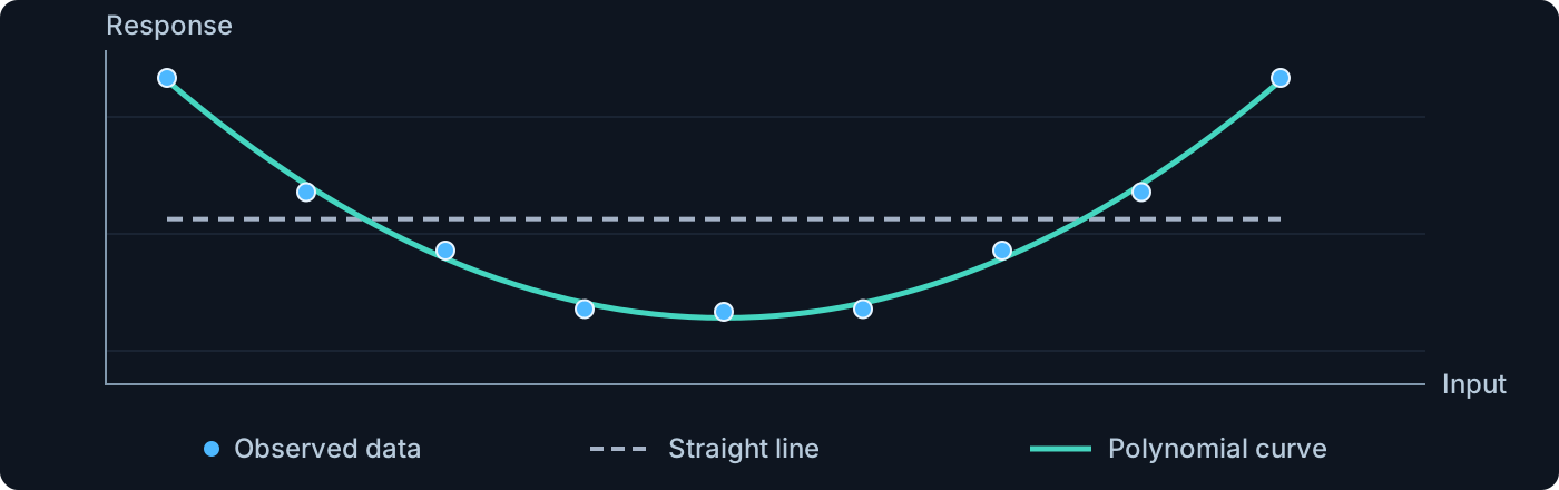
The illustration fits a straight line and a quadratic to the same nine toy observations. The line cannot follow the U-shaped pattern, while the quadratic can. This motivates expanding the feature family. Prediction quality is still assessed on separate data, so extra flexibility is chosen using validation rather than training agreement alone.
Why a polynomial is still linear in its coefficients
“Linear in its parameters” describes how the unknown coefficients enter the prediction rule. For a fixed degree p, the powers 1, x, x², …, xᵖ are known features of each observed input. The model multiplies each feature by one coefficient and adds the resulting terms. Each coefficient occurs to the first power, with no products between unknown coefficients.
For degree 2, the mean prediction is β₀ + β₁x + β₂x². At the known input x = 2, this becomes β₀ × 1 + β₁ × 2 + β₂ × 4. The numbers 1, 2 and 4 are fixed. Estimation changes only their unknown weights. The graph can curve as x changes even though the prediction is a linear weighted sum of the coefficients.
In contrast, a term with a squared unknown coefficient, such as β₁²x, is nonlinear in β₁. Products such as β₁β₂x also break linearity in the original coefficients. The relevant distinction is what happens to the unknown coefficients, not whether the known input has been squared.
This is why polynomial regression can use the linear least-squares machinery: construct the known feature matrix from the chosen powers of x, then multiply it by the unknown coefficient column. The prediction is linear in the coefficient column, while the RSS fitting objective is quadratic because it squares the residual errors.
The degree p is a hyperparameter chosen before each fit. There are p + 1 coefficients, including the intercept. Their allowed space is ℝᵖ⁺¹. Some leading coefficients may be zero, so the fitted curve can have a lower degree than the maximum allowed.
For p = 2 and xᵢ = 2, the features are 1, 2 and 4.
These numbers stay fixed while we fit the β coefficients.
Each coefficient appears only to the first power, as a separate weight on a known feature. The weighted terms are added.
For comparison, is nonlinear in β₁ because the unknown coefficient is squared. Squaring the known input x is allowed.
k = power index, from 0 to p
i = observation index.β₀,…,βₚ = p + 1 learned coefficient weights
xᵢ⁰ = 1 gives the intercept β₀
εᵢ = random error.
Self-check
Consider ŷ = β₀ + β₁x + β₂x². The inputs are known and only the three β coefficients are fitted. Why can this use ordinary linear least squares?
- Because every quadratic curve is also a straight line in x.
- Because squaring x eliminates the need to estimate β₂.
- Because 1, x and x² are known features, each multiplied by one unknown coefficient.
- Because any function of x and β is linear once the data are recorded.
Build one row of polynomial features for each observation
The feature map φ turns one raw predictor into the row [1, xᵢ, xᵢ², …, xᵢᵖ]. Multiplying that row by the coefficient column gives one prediction. For degree 2, input 2 becomes [1, 2, 4]; coefficients (1, 3, −1)ᵀ predict 3. The feature values are fixed while fitting changes their coefficient weights.
Stack these rows to form X. In this lecture X includes the intercept column and any expanded features, so it has p + 1 columns. This differs from a matrix containing only raw predictor measurements. A transformation that learns quantities such as a mean or scale must be fitted on training data only and then applied unchanged to evaluation data.
p = maximum degree.β = coefficient column
X = expanded design matrix, including ones.
All observations become one matrix equation
The design matrix has one row per observation and one column per polynomial power, including the constant column. The target vector y = (y₁, …, yₙ)ᵀ and error vector ε have n entries; β = (β₀, …, βₚ)ᵀ has p + 1 entries. Thus Xβ has the same dimensions as y.
The transpose symbol ᵀ exchanges rows and columns. The equation y = Xβ + ε is just the n individual polynomial observation equations written together. A fitted mean vector is = X. Lowercase bold y denotes the whole response column; yᵢ denotes one recorded response.
y and ε are n-entry columns
β has p + 1 entries.ᵀ = transpose: it swaps rows and columns
ℝ = real numbers.
Fit the coefficients by minimizing the total squared error
Ordinary least squares (OLS) keeps the training inputs and responses fixed and chooses the coefficients. For each candidate coefficient column β, the matrix product Xβ contains its predictions. Subtracting these from the observed-response column y gives the residual column r = y − Xβ. Its i-th entry is yᵢ − .
RSS(β) adds the squares of those residuals. The squared Euclidean norm is exactly the same sum, expressed in vector notation. The notation arg min returns the coefficient column that minimizes the score, whereas min alone would return the smallest score itself. A degree-p polynomial has p + 1 real coefficients, including its intercept, so the search is over ℝᵖ⁺¹. Multiplying the residual row rᵀ by its column r multiplies matching residuals and adds them: rᵀr = ∑ᵢrᵢ². This is the same RSS as the individual-residual sum and the squared norm.
Smaller means a closer fit to the training observations.
We want the coefficient values that give the smallest score.
β = coefficient column, Xβ = predictions
r = y − Xβ = residual column
yᵢ = response i, = prediction i.n = observations, i = case index
p = degree, so β has p + 1 entries
ℝ = real numbers. A hat marks the fitted choice.
ᵀ = transpose: a column becomes a row.
Both rᵀr and ‖y − Xβ‖₂² mean: square each residual, then add.
A three-observation example: the matrix score is still RSS
Use the three training observations (0,1), (1,2) and (2,4). The proposed line 1 + x predicts 1, 2 and 3. The residuals, observed minus predicted, are 0, 0 and 1. Their squared sum is 1. No new error measure has been introduced by writing these numbers in a column.
For any residual column, matrix multiplication gives rᵀr = r₁×r₁ + ⋯ + rₙ×rₙ. Every residual is multiplied by itself, and the products are added. This is the sum of squared residuals, so . The transpose changes the n × 1 column into a 1 × n row, and the product is one number. Here this is 0×0 + 0×0 + 1×1 = 1.
A second candidate, 1 + 1.5x, gives predictions 1, 2.5 and 4, so its residuals are 0, −0.5 and 0 and RSS is 0.25. The exact OLS fit is 5/6 + 1.5x, whose residuals are 1/6, −1/3 and 1/6 and whose RSS is 1/6. The goal is the best score across all coefficient choices, rather than just evaluating one proposed line.
| Input xᵢ | Observed yᵢ | Predicted | Residual rᵢ | rᵢ² |
|---|---|---|---|---|
| 0 | 1 | 1 | 0 | 0 |
| 1 | 2 | 2 | 0 | 0 |
| 2 | 4 | 3 | 1 | 1 |
Transpose it into a row, then multiply matching entries and add.
r = the column of all three residuals.
i = case index, n = observation count (3 here).ᵀ = transpose: a column becomes a row
rᵀr is one number: the total squared error.
Row × column multiplies each residual by itself and adds the results: exactly the definition of RSS.
How do we find the best coefficients ?
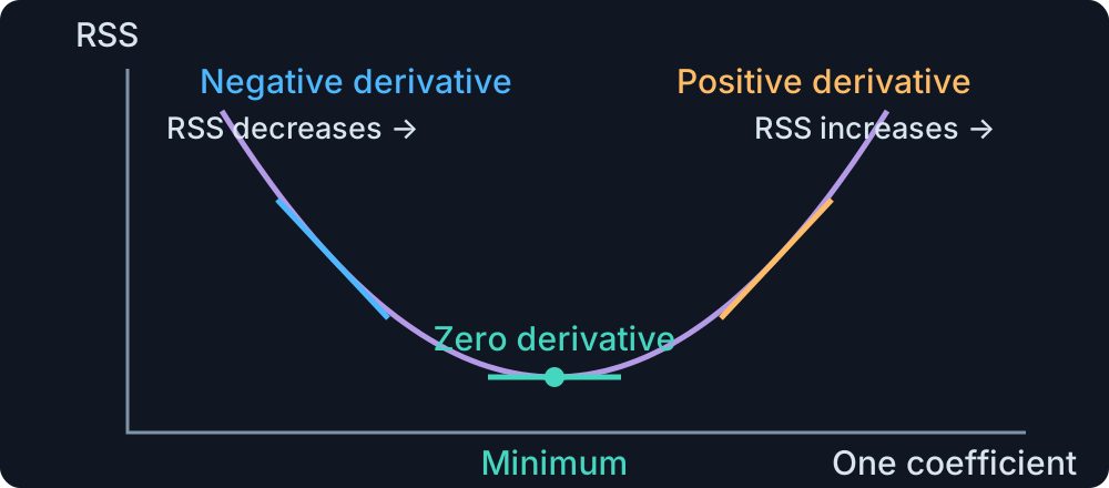
We want to choose the coefficients β that make the sum of squared residuals as small as possible. How can we do that? The notation arg min returns a coefficient vector that attains the smallest RSS. In contrast, min alone returns the numerical value of that smallest RSS. Thus β hat is a set of fitted coefficient values, not an error score. If several coefficient vectors tie for the minimum, any minimizing vector is an OLS solution.
The formula states our goal. Derivatives give us a way to find the coefficient values that achieve it: we look for the bottom of the squared-error surface. The next slide works through the algebra for all coefficients together.
First imagine varying only one coefficient and keeping all other coefficients fixed. The derivative measures the slope of the RSS curve in that direction. A negative derivative means increasing the coefficient initially lowers RSS. A positive derivative means increasing it initially raises RSS. At the bottom, that derivative is zero.
With several coefficients we need to consider every direction at once. The gradient ∇βRSS is the column of partial derivatives with respect to β₀, …, βₚ. Setting this gradient to the zero vector means setting every partial derivative to zero. The graphic shows a one-coefficient slice for intuition; finding the full least-squares solution requires the conditions for all coefficients together.
The least-squares objective is a convex quadratic, meaning its surface is bowl-shaped or has flat directions. There are no separate, worse local minima. Consequently its zero-gradient equations characterize the least-squares minimizers. Flat directions can still give several coefficient choices with the same minimum; the rank condition in the derivation and optional full-column-rank section tells us when the answer is unique.
arg min returns the coefficient values. min alone returns the smallest RSS.
p = polynomial degree
RSS = residual sum of squares. means every coefficient derivative is zero
β = coefficient column
X = fixed feature matrix, y = fixed responses.
Least squares gives a bowl-shaped surface, possibly with a flat valley. Zero gradient finds a minimum, which may have tied coefficient choices.
From squared errors to equations for the coefficients
The task is to turn “minimize RSS” into equations whose unknowns are the coefficients. The data X and y stay fixed throughout the derivation. The first three lines rewrite the same scalar score; differentiation then produces the conditions a fitted coefficient vector must satisfy.
Expanding (y − Xβ)ᵀ(y − Xβ) gives four terms. The identity (AB)ᵀ = BᵀAᵀ is used to put them into a consistent order. In particular, yᵀXβ is a 1 × 1 scalar, so it equals its transpose βᵀXᵀy. The two cross terms therefore combine into −2βᵀXᵀy.
Differentiate with respect to β. The term yᵀy is constant and contributes zero. The linear term contributes −2Xᵀy. The quadratic term βᵀXᵀXβ contributes 2XᵀXβ because XᵀX is symmetric. These are the vector versions of a constant having derivative zero, a linear term having a constant derivative, and a square producing a factor two.
At a minimum set −2Xᵀy + 2XᵀX equal to zero. Move the first term to the other side and divide by two. The result, XᵀX = Xᵀy, is the system of normal equations. Because RSS is a convex quadratic, its solutions minimize RSS. Whether the coefficient vector is unique is a separate question, addressed next.
Finally, if XᵀX is invertible, multiply both sides of the normal equations on the left by (XᵀX)⁻¹. The product (XᵀX)⁻¹(XᵀX) is the identity matrix: the matrix equivalent of multiplying by one. It leaves the coefficient vector unchanged, so the left side becomes the fitted coefficient vector by itself. The right side becomes (XᵀX)⁻¹Xᵀy. This inverse formula requires independent feature columns; no feature column is a linear combination of the others.
1 · Write the score. The residual column becomes a row times a column. This adds the squared errors.
2 · Expand both brackets. Keep the order of matrix factors. The two middle terms turn out to be equal numbers.
3 · Combine the middle terms. Since yᵀXβ = βᵀXᵀy, they add to −2βᵀXᵀy. This is the matrix version of expanding a square.
4 · Differentiate only β. X and y are fixed. The constant term vanishes, and the quadratic term contributes the factor 2.
5 · Set every derivative to zero, divide by 2 and rearrange. These are the normal equations for the least-squares coefficients.
6 · Final result, when XᵀX is invertible. Multiply both sides on the left by its inverse to isolate the coefficients.
The matrix is the Moore–Penrose pseudoinverse.
β = candidate coefficients, = fitted coefficients
∇β = differentiate with respect to all coefficients.(AB)ᵀ = BᵀAᵀ for compatible matrices A and B
yᵀXβ is one number, unchanged by transposing
X⁺ = Moore–Penrose pseudoinverse.
−1 = matrix inverse, requiring independent columns.
When XᵀX is invertible, the Moore–Penrose pseudoinverse is X⁺ = (XᵀX)⁻¹Xᵀ, so the fitted coefficient vector can be written as X⁺y. Invertibility is required for this particular inverse expression. A least-squares solution and the Moore–Penrose pseudoinverse still exist when X has dependent columns, although the minimizing coefficients may not be unique.
The polynomial degree p is a hyperparameter: it sets the allowed powers before coefficients are fitted. We next compare polynomial regression across different degrees, inspecting training fit and prediction on held-out observations. Degree selection uses validation evidence, with a separate final test assessment.
The degree p is a hyperparameter: choose it before fitting. Next, compare polynomial models across different degrees.
When does the inverse formula give one coefficient choice?
Optional reading: this expands the full-column-rank and pseudoinverse explanation from the coefficient derivation. It is additional detail for independent reading.
Starting from XᵀX = Xᵀy, we can multiply both sides by (XᵀX)⁻¹ if that inverse exists. This gives the familiar closed-form OLS expression. The inverse exists exactly when no feature column of X is a linear combination of its other columns: X has full column rank. For a degree-p polynomial this requires enough distinct input values to identify its p + 1 coefficients.
“Scaled copies” means multiplying whole columns by fixed numbers and adding them. Sharing a raw input does not automatically make polynomial columns dependent. For x values 0, 1 and 2, the columns 1, x and x² contain different patterns: no fixed combination of 1 and x equals x² across all three rows.
Dependent columns repeat information. For example, a model containing x twice has the expression β₀ + β₁x + β₂x = β₀ + (β₁ + β₂)x. The slope pairs (2,3) and (5,0), with the same intercept, give identical predictions at every input. The observations can determine the combined slope without determining each separate coefficient.
Least-squares solutions still exist in this situation, but several coefficient columns can give the same minimum RSS and the same fitted training values. The Moore–Penrose pseudoinverse X⁺ selects the tied coefficient vector with the smallest sum of squared entries. Its full-column-rank form is (XᵀX)⁻¹Xᵀ. This distinguishes an unavailable inverse formula from a nonexistent least-squares fit.
In numerical work use a least-squares solver. Common methods use QR factorization or singular value decomposition (SVD) rather than explicitly forming a matrix inverse. These numerical methods are implementation details; the lecture’s main distinction is between finding a minimum and having one unique coefficient vector.
No feature column is an exact sum of scaled copies of the others. This is full column rank.
Multiply both sides of the normal equations by (XᵀX)⁻¹ to isolate the coefficients.
Imagine including the same x column twice. Only the sum of its two coefficients affects predictions.
The pairs (2,3) and (5,0) cannot be distinguished from the predictions.
= fitted coefficient column
ᵀ = transpose, −1 = matrix inverse.
x = the input repeated in the example. also handles tied solutions
X⁺ = Moore–Penrose pseudoinverse
It selects the tied solution with the smallest sum of squared coefficients.
The inverse formula needs independent columns. Least-squares fitting still works when coefficients are not unique.
Choose the degree, then fit the coefficients
A hyperparameter defines a choice about the model family before a candidate model is trained. Polynomial degree p decides which powers of the input appear and therefore which shapes are possible. With p = 1, OLS estimates an intercept and a slope. With p = 2, OLS estimates those plus the coefficient of x². The coefficients are parameters learned from the training observations.
To compare degrees, choose one candidate degree, fit its coefficients on training data and measure validation error. Repeat for the other candidate degrees. Select a suitable degree using validation or cross-validation, then assess the fixed procedure on the final test set. Cross-validation repeats the training/validation comparison over several splits.
With exact unregularized least squares, increasing the permitted degree cannot increase the best attainable training RSS, since setting the extra coefficients to zero recovers the simpler model. This makes training RSS alone unsuitable for choosing degree. A more flexible curve may follow training noise and predict new observations worse, which leads into the overfitting examples.
OLS fits two numbers: β₀ and β₁.
OLS fits three numbers: β₀, β₁ and β₂.
β = coefficient column, including intercept β₀.x = input, f(x) = model’s prediction
A degree-p model has p + 1 coefficients.
A lower training RSS alone does not justify a higher degree. Use validation for the choice and keep the test set for final assessment.
Overfitting and underfitting: what can go wrong?
Overfitting occurs when a model adapts to noise or sample-specific fluctuations in the training observations instead of capturing only relationships that transfer to new observations. A more flexible polynomial can fit the training points more closely while making less reliable predictions between points or near the edges. A strong training score alone therefore does not establish good generalization.
Underfitting occurs when the model family cannot represent the main signal in the data. For example, constant or linear models can miss the curvature in a relationship that a quadratic model can capture. In this case the model fails to explain a systematic pattern even in its training observations.
Model complexity describes the flexibility of the prediction family. In polynomial regression, the degree controls this flexibility. Too little flexibility can cause underfitting. More flexibility can represent the signal better, but can also follow training noise and cause overfitting. These are tendencies, rather than diagnoses based on degree alone.
Fit each candidate degree on training observations, then compare its prediction error on validation observations or by cross-validation. Keep the final test set for assessing the selected procedure. The following examples first illustrate overfitting with degrees 1, 5, 15 and 23, then underfitting with degrees 0, 1 and 2. Part 2 explains the related bias–variance reasoning.
The model fits sample-specific fluctuations in the training data that do not carry over to new cases.
Typical clue: better training fit, worse held-out prediction.
Example: a very flexible polynomial follows small wiggles.
The model is too restrictive to represent the main pattern, even in the training data.
Typical clue: a clear pattern remains unexplained.
Example: a straight line misses a curved relationship.
Increasing flexibility can reduce underfitting but may lead to overfitting. Compare validation performance to choose the polynomial degree.
Overfitting: a flexible curve can follow training noise
Self-check
On the same split, degree 1 has training/validation RMSE (0.10, 0.12); degree 15 has (0.04, 0.30). What is the best next decision for prediction?
- Choose degree 15 because its training error is smaller.
- Choose degree 15 because more coefficients guarantee better generalization.
- Use the final test set repeatedly until one degree has the smallest score.
- Prefer degree 1 using validation evidence, then assess the fixed choice on an untouched test set.
Overfitting occurs when a model adapts to noise or sample-specific fluctuations in the training observations instead of capturing only relationships that transfer to new observations. A more flexible polynomial can fit the training points more closely while making less reliable predictions between points or near the edges. A strong training score alone therefore does not establish good generalization.
Compare illustrative degree-1, 5, 15 and 23 curves on the same training and held-out points. A flexible curve can follow small training fluctuations and behave poorly between points or near the edges. Zoom and toggle curves to inspect that behavior.
The displayed score table describes these particular supplied curves. At very high degrees, numerical rank, basis and solver choices can substantially affect the fitted curve. Do not interpret one table as a universal error for every degree-23 OLS implementation. For choosing a degree, use validation rather than repeatedly selecting on a final test.
Try it: Overfitting means learning training details that do not generalize. Compare degrees 1, 5, 15 and 23: inspect the wiggles and the held-out errors.

Static preview. Open handout.html to use the interactive example.
Overfitting: better training fit, worse prediction
In this illustrative comparison, training R² increases from 0.9850 to 0.9938 while held-out RMSE increases from 0.1220 to 0.3052. Thus closer agreement with training observations does not guarantee better prediction. Compare both columns before deciding what to investigate.
These metrics describe the supplied candidate curves. The exact numerical fitting method for the highest-degree curve is unspecified, so the table should not be used as a numerical reference for a different implementation. Overfitting means learning sample-specific variation that does not transfer; it is diagnosed using an appropriate evaluation design, not degree alone.
| Degree | Training R² · illustrative curves | Held-out RMSE · illustrative curves |
|---|---|---|
| 1 | 0.9850 | 0.1220 |
| 5 | 0.9878 | 0.1225 |
| 15 | 0.9933 | 0.1548 |
| 23 | 0.9938 | 0.3052 |
Read each row as one supplied curve evaluated on the same split. Training R² is unit-free. Held-out RMSE uses the response scale. The intermediate degrees also show why improving training fit alone is insufficient.
Underfitting: a simple model misses the main pattern
Underfitting occurs when a model family is too restrictive to capture the main signal, even in the training observations.
Compare degree 0, 1 and 2 on a curved dataset. Degree 0 predicts a constant, degree 1 a line and degree 2 a quadratic. All observations remain visible over the full response range. The quadratic can represent the main curvature that the simpler families miss.
For a selected degree, training R² and test RMSE are calculated from its fit. RSE uses n − (p + 1), assuming full rank and positive residual degrees of freedom. Degree-0, 1 and 2 fits therefore use different residual denominators even though they use the same training cases.
Try it: Underfitting means the family is too restrictive to capture the signal. Compare p = 0 (constant), 1 (line) and 2 (quadratic) on these curved data.

Static preview. Open handout.html to use the interactive example.
Recognize underfitting and overfitting from the evidence
Poor training fit can indicate a family too restrictive to represent the signal. It can also reflect unsuitable features, bad measurements or an optimization failure. Strong training fit accompanied by weak held-out performance is compatible with overfitting.
A poor held-out score is not a complete diagnosis: inspect distribution change, leakage, grouping and whether the split represents the intended use. Use both the numerical scores and residual patterns to choose the next check.
Before you leave this part
- Interpret the intercept, slope and residuals of a line.
- Explain what a fit score does and does not establish.
- Recognize overfitting and underfitting from training and held-out behavior.
Explain the current lecture’s central distinctions using a concrete example. In Part 1, separate a candidate line, its fitted coefficients, training fit and unseen-case performance. In Part 2, distinguish sample sensitivity, statistical uncertainty and causal interpretation.
Use an interactive example to support the explanation. State the observation set, symbols, metric and assumptions that make the numerical claim meaningful.
Five metrics: what does each one tell me?
A residual is an observed response minus the model’s prediction at the same input. RSS, the residual sum of squares, squares each training residual and adds the results. It is the total squared training error, so its value depends on the number of cases and the response units. Compare it on the same observations.
TSS, the total sum of squares, measures response variation around the mean. It is the squared error of a reference predictor that always returns that mean. It describes the data’s variation before asking how much the fitted model explains.
RSE, residual standard error, estimates the spread of the model’s unexplained random error, in response units. For a simple line it is the square root of the whole ratio RSS/(n − 2), allowing for fitting the intercept and slope. It is a training-based estimate of error spread, rather than a test-set prediction score.
R², the coefficient of determination, compares the model’s squared error with TSS. A value of 1 means no residual error, 0 means the same squared error as the mean-only baseline, and a negative value means worse than that baseline. The score requires nonzero TSS. It is not a percentage of predictions that are correct.
Test RMSE, root mean squared error, measures the size of prediction mistakes on observations not used to fit or choose the model. Square the test errors, average them and take the square root. This returns the score to response units and gives larger misses more influence. RSE describes estimated training noise; test RMSE assesses the fixed model’s prediction on new cases.
Ordinary least squares (OLS) estimates coefficients by minimizing RSS. Use validation to compare model choices and a final test set to assess the selected procedure. Underfitting misses a stable pattern, while overfitting follows training details that do not transfer. Repeating training on new samples lets us study model variability.
| Metric | Formula | What does it show me? |
|---|---|---|
| RSSResidual sum of squares | Training misses, squared and added. Smaller means a closer fit to the same cases. | |
| TSSTotal sum of squares | Squared misses from always predicting the response average: the variation available to explain. | |
| RSEResidual standard error | Estimated scatter around the fitted model, in response units (such as kg). | |
| R²Coefficient of determination | Improvement over the average baseline: 1 = perfect, 0 = equal, negative = worse. | |
| Test RMSERoot mean squared error | Typical size of mistakes on new test cases, in response units. Large misses count more. |
= observed response, = prediction
= response mean used for TSS. = training count, = test count
= independent fitted coefficients, including the intercept
For a line . RSE needs . R² needs .
The RSE formula uses for the number of independently fitted coefficients, including the intercept. For a straight line , so the denominator is . For a polynomial of degree with independent feature columns, . RSE requires positive residual degrees of freedom, . The R² ratio requires .
In the test-RMSE row, the observed responses and predictions belong to the held-out test set, and is its number of cases. The residuals in RSS and the mean in TSS describe the training observations in this recap.
Further reading and practice
For further explanation of linear regression, read Chapter 3 of An Introduction to Statistical Learning. Penn State STAT 501 develops assumptions and inference in more detail. NumPy least squares explains numerical solutions and rank.
The local interactive examples connect formulas with predictions and residuals. Use them to reproduce calculations, keeping training fit, unseen-case performance and causal claims distinct.
Notation reference
| Symbol | Meaning |
|---|---|
| i, n | Observation index and number of training observations. |
| xᵢ, yᵢ | Recorded input and response for observation i. |
| X, Y (plain) | Input and response random variables; values are written in lowercase. |
| , rᵢ | Fitted prediction and residual: rᵢ = yᵢ − . |
| β₀, β₁ | Intercept and slope of a simple linear mean model. |
| , | Estimated coefficient vector and its j-th estimated coefficient; a hat marks estimation. |
| β (bold) | Column of model coefficients, including the intercept. |
| εᵢ, ε (bold) | Unobserved random error of one response and the column of all errors. |
| , | Sample means of the stated observations. |
| RSS, TSS | Residual sum of squares and total sum of squares around a response mean. |
| MSE, RMSE | Mean squared prediction error and its square root on a stated set. |
| R² | Coefficient of determination: 1 − RSS/TSS, for TSS > 0. |
| , q | is the test-case count in test RMSE. q is the independent fitted coefficient count, including the intercept. |
| RSE | Residual standard error; RSE² estimates common error variance under the assumptions. |
| p, k | Maximum polynomial degree and power index k = 0,…,p. |
| φ(xᵢ) | Feature row [1, xᵢ, …, xᵢᵖ]. |
| X (bold), y (bold) | Expanded design matrix and response column; polynomial X has n × (p + 1) entries. |
| m, j | Number of predictors and predictor index in a multiple-regression model. |
| ᵀ, −1, X⁺ | Transpose, matrix inverse and Moore–Penrose pseudoinverse. |
| ℝ, ℝᵈ | Real numbers and columns containing d real entries; d is a dimension. |
| ∑, ‖v‖₂² | Sum over the stated index; sum of squared entries of vector v. |
| arg min, min, ∇ | Minimizing argument, minimum objective value, and vector of coefficient derivatives. |
| c | Common input value in the constant-input example. |
| E[ε | X] | Conditional mean error, assumed zero to interpret the line as a mean response. |
The slope of RSS as one coefficient changes, keeping the others fixed.
The list of these derivatives: one for every coefficient.
Every derivative is zero. The gradient is the zero vector.