Artificial Intelligence and Machine Learning · Lecture 09 of 16

Regression · Part 1

Fitting and evaluating prediction models

Fit numerical predictions and compare simple and flexible models using both training and held-out evidence.

01Linear regression
02Training
03Model evaluation
04Polynomial regression
Regression · Part 1

From observations to a fitted prediction rule

Observe → choose a family → fit coefficients → check new-case predictions.

01 · Linear regression

Describe the data and a line

03 · Model evaluation

Measure fit and unseen error

04 · Polynomial regression

Add features and compare flexibility

01 · Linear regression

Inspect 25 fertilizer and yield observations

Each dot is one trial: input x = fertilizer, response y = yield. Select a point, zoom or pan to inspect the trend.

01 · Linear regression

Start with a line as an approximate prediction rule

Simple linear regression uses one input to describe a numerical response. We choose a family of straight lines and will learn which line fits the observations.

yi≈f(xi)=β0+β1xi
What we observe

For each trial i, record input xᵢ and response yᵢ.
Example: fertilizer level and measured yield.

What the line describes

f(xᵢ) is the line’s response at input xᵢ.
β₀ sets its height; β₁ controls its slope.

i = trial index
n = number of training trials
f = prediction function.
≈ means “approximately equal”: the observations need not lie exactly on the line.
01 · Linear regression

The same input can give different observed responses

Intercept β₀ = 1

At x = 0, the line’s mean response is 1. This is where the line meets the vertical axis.

Slope β₁ = 3

At x = 2, the mean is 7; at x = 3, it is 10: an increase of 3. Actual responses can lie above or below those means, so two measured yields need not differ by 3.

For the toy mean line f(x)=1+3x, input 2 has mean response 7, while two observed responses are 6 and 8.
f(2)=1+3×2=7

Both observations have x = 2. One response is 1 above the line and the other is 1 below it. The line summarizes the typical response, rather than predicting each case perfectly.

01 · Linear regression

Make the approximation explicit: add a random error

Instead of saying only “the response is near a line”, separate the line’s systematic part from the random variation of each observation.

Systematic part: the line
f(xi)=β0+β1xi

Describes how the mean response changes with x.
The coefficients β₀ and β₁ are unknown.

Observed response: line + error
yi=β0+β1xi+εi

εᵢ (epsilon) is the deviation of observation i from that mean. It includes unexplained variation, not just measurement mistakes.

Adding εᵢ makes the observation equation exact. It does not make the line’s predictions perfect.

02 · Training

A residual measures one prediction’s vertical miss

Before comparing whole lines, measure how far one prediction is from its observed response.

ri=yi−yˆi
One concrete case

Observed yield yᵢ = 8; current prediction yˆi = 7.
The residual is 8 − 7 = +1: the line predicts too low.

Read the sign

Positive residual: observation above the line.
Negative residual: observation below the line.
Zero residual: this prediction is exact.

i = observation index
yᵢ = observed response
yˆi = the current line’s prediction.
A residual is a vertical response difference at the same input xᵢ, not a perpendicular distance.
02 · Training

We need one score to compare candidate lines

Moving or tilting a line improves some predictions and worsens others. We need a guiding rule that combines all of their misses.

Candidate A: larger misses

Residuals: +2 and −2.
The signed sum is 0, but neither prediction is exact.
Squared misses: 4 + 4 = 8.

Candidate B: smaller misses

Residuals: +1 and −1.
The signed sum is also 0.
Squared misses: 1 + 1 = 2.

Residual sum of squares (RSS): square each residual, then add. Candidate B has the smaller score on these same cases.

Squaring stops positive and negative misses from canceling.Larger misses receive more weight: doubling a residual makes its square four times larger.
02 · Training

Least squares adds the squared vertical gaps

yˆi=β0+β1xiri=yi−yˆi
RSS(β)=∑i=1nri2=∑i=1n(yi−β0−β1xi)2

Residuals +2 and −2 cancel when added, but contribute 4 + 4 = 8 to RSS.

β = (β₀, β₁)ᵀ = candidate coefficients
n = training count.
yˆi = prediction
rᵢ = observed minus predicted
RSS = residual sum of squares.
02 · Training

Training means choosing the coefficients with the smallest RSS

Ordinary least squares (OLS) is a fitting rule: choose the coefficients that make the sum of squared prediction errors (RSS) as small as possible.

βˆ=arg minβ∈ℝ2RSS(β)
Why “ordinary”?

Every squared residual has the same weight.
Fit β₀ and β₁, keeping the observations fixed.

What is returned?

arg min returns the best coefficients.
min returns the smallest error value.

β = candidate coefficient pair
βˆ = fitted coefficient pair.
ℝ² = all pairs of real numbers
OLS = ordinary least squares.
02 · Training

Move the line and watch the residuals change

β₀ moves the line up or down; β₁ changes its slope. Watch the residuals, then press Fit OLS to minimize RSS.

02 · Training

Where do the slope and intercept formulas come from?

They solve the OLS problem: minimize RSS. Differentiate RSS with respect to β₀ and β₁, set both derivatives to zero, then solve the two equations.

βˆ1=∑i=1n(xi−x¯)(yi−y¯)∑i=1n(xi−x¯)2
βˆ0=y¯−βˆ1x¯
x¯ = (1/n)∑xᵢ
y¯ = (1/n)∑yᵢ: training sample means.
βˆ1 = fitted slope
βˆ0 = fitted intercept
all sums use i = 1,…,n.
02 · Training

When do the data determine one best-fitting line?

To learn a slope, we need observations at different input values. Here x is the input and y is the observed response.

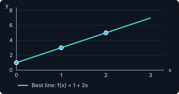
Different inputs: one best line

Trials use x = 0, 1 and 2.

Three observations at (0,1), (1,3), (2,5) lie on the unique best line f(x)=1+2x.

The best slope is 2 and the intercept is 1.
Tilting or shifting this line increases RSS.

Same input: tied best lines

All three trials use x = 2. Their responses are 4, 5 and 6.
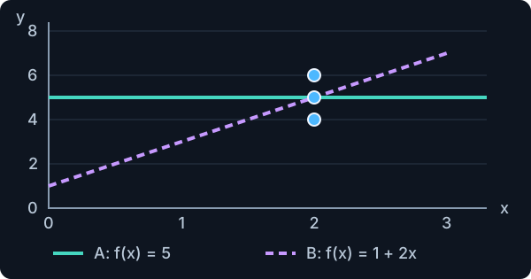
Three observations at x=2 have responses 4,5,6. A horizontal line at y=5 and the line f(x)=1+2x both predict 5 there.

Both lines predict 5 at x = 2 and have RSS = 2.
These trials cannot tell us which slope to choose.

A best fit can exist without a unique line. If every trial uses the same input, we cannot separate the effects of slope and intercept.

02 · Training

Compare a candidate line with the exact OLS fit

A candidate is a proposed line. We deliberately start with f(x) = 2 + 2x. Press Show OLS best fit to see how minimizing RSS improves this guess.

03 · Model evaluation

Model evaluation: what does a good score tell us?

Evaluation uses one or more metrics to assess particular aspects of model quality, such as predictive ability or robustness to noise.

Scores need interpretation

Evaluation can hide pitfalls. A result depends on the metric, the data and how the evaluation was performed.

Interpreting the numbers takes care and experience.

Our focus in this lecture

Explaining the data: how well does the model describe the observations?

Generalizing: how well does it predict new instances?

We begin with two popular linear-regression metrics: residual standard error (RSE) and coefficient of determination (R²).

First assess the fit to the observed data.Then check prediction on held-out cases: observations not used for fitting.
03 · Model evaluation · Training performance

Training performance: how closely does the line fit?

Training performance describes agreement with the observations used for fitting. RSE summarizes the remaining errors in response units.

RSE=RSSn−2=∑i=1n(yi−yˆi)2n−2
Why divide by n − 2?

The line’s height and tilt were chosen using these same observations, making training errors look optimistic. The n − 2 correction accounts for estimating those two coefficients.

How do we read the scale?

On the same observations, a lower RSE means closer predictions. RSE = 2 kg estimates an error standard deviation of 2 kg.

RSS = training residual sum of squares
n = number of training observations
i = observation index, from 1 to n.
yᵢ = observed response
yˆi = fitted line’s prediction
Require n > 2, varying inputs and the stated linear-model assumptions.

RSE ≥ 0 has no fixed upper bound. Its absolute size needs context: is an error scale of 2 kg large for this task?

03 · Model evaluation · Training performance

From RSE to R²: why use a relative measure?

RSE is an absolute measure. Its numerical value alone can be difficult to interpret: when does it indicate a good model?

RSE · an absolute error scale
RSE∈[0,∞)

There is no fixed upper bound.
A “good” RSE depends on the response units, its scale and the task.

2 kg=2000 g

Same error scale, different units.

R² statistic · coefficient of determination

Compare the model’s squared errors with a baseline that always predicts the response mean.
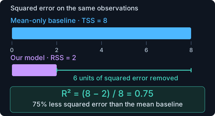
TSS is 8, RSS is 2, and their reduction of 6 out of 8 gives R squared equal to 0.75.

TSS = baseline error. RSS = model error.
R² compares the improvement with the baseline.

RSE asks “How large are the errors?” R² asks “How much better is this model than predicting the mean?”

03 · Model evaluation · Training performance

R²: compare the model with a mean-only baseline

The baseline and the relative score

The baseline always predicts y¯: intercept β0=y¯ and slope β₁ = 0.

TSS=∑i=1n(yi−y¯)2
R2=TSS−RSSTSS=1−RSSTSS
R2=1−∑i=1n(yi−yˆi)2∑i=1n(yi−y¯)2

TSS = total sum of squares around the mean.
RSS = sum of squared model prediction errors.

How to read R² · require TSS > 0
R² = 1 · perfect fit

RSS = 0: every prediction matches its observed response.

R² = 0 · matches the baseline

RSS = TSS: the same squared error as always predicting the mean.

R² < 0 · worse than the baseline

RSS > TSS: more squared error than the mean-only predictor.

Range: −∞ < R² ≤ 1.
Training OLS with an intercept gives R² ≥ 0.
On held-out data, negative R² can be a valid result.

yᵢ = observed response
yˆi = model prediction, y¯ = response mean
n = number of cases, i = case index.
No universal “good” threshold: it depends on the task and field.
Outliers (points far from the pattern) can change the score.
Example: RSS = 2, TSS = 8 → R² = 0.75.
03 · Model evaluation · Test performance

Good training fit does not guarantee good prediction

Training fit describes the data used for estimation. To assess prediction on new instances, keep separate data for validation and final testing.

Train

Estimate coefficients and preprocessing.

Validate

Compare model families and degrees.

Test

Assess the final chosen procedure.

Use time-aware or group-aware splits when those reflect the real prediction task.

03 · Model evaluation · Test performance

Test performance: root mean squared error (RMSE)

Here we use RMSE as a test-performance metric. Keep the fitted model fixed and compare its predictions with responses in a separate test set.

RMSE=1ntest∑i=1ntest(yi−yˆi)2
The three operations

1. Square each test prediction error.
2. Average over the ntest test cases.
3. Take the square root to return to response units.

A separate toy test set

Test responses: (3, 5, 7). Predictions: (4, 5, 6).
Squared errors: 1, 0, 1. ntest = 3.
Test RMSE = √(2/3) ≈ 0.82.

RMSE = root mean squared error
ntest = number of test cases
n = number of training cases.
yᵢ = observed test response
yˆi = fixed model prediction for test case i.

The test data do not fit or select the model. Average over ntest test cases, with no n − 2 adjustment. A lower test RMSE means smaller test prediction errors.

03 · Model evaluation · Test performance

Compare training and test RMSE for a fixed model

The fixed model is scored on 25 training cases and 10 test cases. Test RMSE assesses prediction on unseen cases. The test responses never change the coefficients.

03 · Model evaluation

Recap: which question does each score answer?

For a fitted line, keep training fit, estimated noise and prediction on new test cases separate.

RSS

Residual sum of squares
RSS=∑i=1nri2

Total squared prediction error on the training data.

RSE

Residual standard error
RSE=RSSn−2

Estimated error standard deviation, in response units.

R²

Coefficient of determination
R2=1−RSSTSS

Improvement over always predicting the response mean.

Test RMSE

Root mean squared error
Test RMSE=RSStestntest

Prediction error on unseen test cases, in response units.

rᵢ = observed minus predicted training response
n = number of training cases
ntest = number of test cases.
RSStest = sum of squared test errors
TSS = squared error of the mean-only baseline
R² requires TSS > 0.
04 · Polynomial regression

Polynomial regression lets the model follow curved patterns that a straight line would miss.
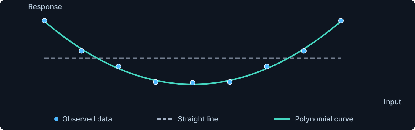
On the same U-shaped observations, a polynomial curve follows the pattern while the straight line misses it.
04 · Polynomial regression

Why a polynomial is still linear in its coefficients

Choose the degree p first. The input and its powers are known numbers. We learn the coefficients that weight those numbers.

yi=∑k=0pβkxik+εi
Known input → known numbers

For p = 2 and xᵢ = 2, the features are 1, 2 and 4.

Prediction=β0×1+β1×2+β2×4

These numbers stay fixed while we fit the β coefficients.

Why the parameters enter linearly

Each coefficient appears only to the first power, as a separate weight on a known feature. The weighted terms are added.

For comparison, β12x is nonlinear in β₁ because the unknown coefficient is squared. Squaring the known input x is allowed.

p = chosen maximum degree
k = power index, from 0 to p
i = observation index.
β₀,…,βₚ = p + 1 learned coefficient weights
xᵢ⁰ = 1 gives the intercept β₀
εᵢ = random error.
04 · Polynomial regression

Build one row of polynomial features for each observation

φ(xi)=[1xixi2…xip]
Known features × learned coefficients

If xᵢ = 2, the feature row is [1, 2, 4].
With β = (1, 3, −1)ᵀ, prediction = 1 + 6 − 4 = 3.
The feature values 1, 2 and 4 are fixed numbers, not extra unknowns.

Stack the observations

X has n rows and p + 1 columns.
Each column is one power: 1, x, x², …, xᵖ.

φ(xᵢ) = feature row for observation i
p = maximum degree.
β = coefficient column
X = expanded design matrix, including ones.
04 · Polynomial regression

All observations become one matrix equation

X=[1x1…x1p1x2…x2p⋮⋮⋱⋮1xn…xnp]
y=[y1⋮yn]
β=[β0⋮βp]
y=Xβ+ε
X ∈ ℝⁿˣ⁽ᵖ⁺¹⁾
y and ε are n-entry columns
β has p + 1 entries.
ᵀ = transpose: it swaps rows and columns
ℝ = real numbers.

The i-th entry of Xβ is exactly β₀ + β₁xᵢ + ⋯ + βₚxᵢᵖ.

04 · Polynomial regression

Fit the coefficients by minimizing the total squared error

Keep the observations fixed. Change the coefficients to make predictions as close as possible to the observed responses.

RSS(β)=∑i=1n(yi−yˆi)2=rTr=‖y−Xβ‖22
βˆ=arg minβ∈ℝp+1RSS(β)
RSS: residual sum of squares

Smaller means a closer fit to the training observations.

arg min: return the coefficients

We want the coefficient values that give the smallest score.

y = observed responses, X = feature matrix
β = coefficient column, Xβ = predictions
r = y − Xβ = residual column
yᵢ = response i, yˆi = prediction i.
n = observations, i = case index
p = degree, so β has p + 1 entries
ℝ = real numbers. A hat marks the fitted choice.
ᵀ = transpose: a column becomes a row.

Both rᵀr and ‖y − Xβ‖₂² mean: square each residual, then add.

04 · Polynomial regression

A three-observation example: the matrix score is still RSS

Try the proposed line yˆi=1+xi. Here β₀ = 1 and β₁ = 1. These are candidate values, before fitting.

Input xᵢObserved yᵢPredicted yˆiResidual rᵢrᵢ²
01100
12200
24311
The same residuals as a column
r=[001]

Transpose it into a row, then multiply matching entries and add.

RSS=rTr=[001][001]=02+02+12=1
rᵢ = yᵢ − yˆi is one residual
r = the column of all three residuals.
i = case index, n = observation count (3 here).
ᵀ = transpose: a column becomes a row
rᵀr is one number: the total squared error.

RSS=∑i=1nri2=rTr
Row × column multiplies each residual by itself and adds the results: exactly the definition of RSS.

04 · Polynomial regression

How do we find the best coefficients β?

We want to choose the coefficients β that make the sum of squared residuals as small as possible. How can we do that?

βˆ=arg minβRSS(β)=arg minβ‖y−Xβ‖22

arg min returns the coefficient values. min alone returns the smallest RSS.
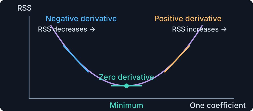
A bowl-shaped error curve: negative slope on the left, zero slope at the minimum, and positive slope on the right
One derivative

The slope of RSS as one coefficient changes, keeping the others fixed.

The gradient ∇

The list of these derivatives: one for every coefficient.

At a least-squares minimum

Every derivative is zero. The gradient is the zero vector.

βⱼ = coefficient j, with j = 0,…,p
p = polynomial degree
RSS = residual sum of squares.
∇βRSS(β)=0 means every coefficient derivative is zero
β = coefficient column
X = fixed feature matrix, y = fixed responses.

Least squares gives a bowl-shaped surface, possibly with a flat valley. Zero gradient finds a minimum, which may have tied coefficient choices.

04 · Polynomial regression

From squared errors to equations for the coefficients

RSS(β)=(y−Xβ)T(y−Xβ)

1 · Write the score. The residual column becomes a row times a column. This adds the squared errors.

RSS(β)=yTy−yTXβ−βTXTy+βTXTXβ

2 · Expand both brackets. Keep the order of matrix factors. The two middle terms turn out to be equal numbers.

RSS(β)=yTy−2βTXTy+βTXTXβ

3 · Combine the middle terms. Since yᵀXβ = βᵀXᵀy, they add to −2βᵀXᵀy. This is the matrix version of expanding a square.

∇βRSS(β)=−2XTy+2XTXβ

4 · Differentiate only β. X and y are fixed. The constant term vanishes, and the quadratic term contributes the factor 2.

XTXβˆ=XTy

5 · Set every derivative to zero, divide by 2 and rearrange. These are the normal equations for the least-squares coefficients.

βˆ=(XTX)−1XTy=X+y

6 · Final result, when XᵀX is invertible. Multiply both sides on the left by its inverse to isolate the coefficients.
The matrix X+=(XTX)−1XT is the Moore–Penrose pseudoinverse.

X = fixed feature matrix, y = observed responses
β = candidate coefficients, βˆ = fitted coefficients
∇β = differentiate with respect to all coefficients.
(AB)ᵀ = BᵀAᵀ for compatible matrices A and B
yᵀXβ is one number, unchanged by transposing
X⁺ = Moore–Penrose pseudoinverse.
−1 = matrix inverse, requiring independent columns.

The degree p is a hyperparameter: choose it before fitting. Next, compare polynomial models across different degrees.

04 · Polynomial regression

Choose the degree, then fit the coefficients

The degree decides which shapes are allowed. Training chooses the best coefficients within that choice.

Choose p = 1: allow a straight line
f(x)=β0+β1x

OLS fits two numbers: β₀ and β₁.

Choose p = 2: also allow curvature
f(x)=β0+β1x+β2x2

OLS fits three numbers: β₀, β₁ and β₂.

1 · Choose a candidate degreeThis is the hyperparameter p.
2 · Fit its coefficientsThese are the learned parameters β.
3 · Compare validation errorUse it to choose a suitable degree.
p = maximum polynomial degree
β = coefficient column, including intercept β₀.
x = input, f(x) = model’s prediction
A degree-p model has p + 1 coefficients.

A lower training RSS alone does not justify a higher degree. Use validation for the choice and keep the test set for final assessment.

04 · Polynomial regression

Overfitting and underfitting: what can go wrong?

A model should learn stable patterns that also work on new observations. Its flexibility can create two different problems.

Overfitting · learning the noise

The model fits sample-specific fluctuations in the training data that do not carry over to new cases.

Typical clue: better training fit, worse held-out prediction.
Example: a very flexible polynomial follows small wiggles.

Underfitting · missing the signal

The model is too restrictive to represent the main pattern, even in the training data.

Typical clue: a clear pattern remains unexplained.
Example: a straight line misses a curved relationship.

Increasing flexibility can reduce underfitting but may lead to overfitting. Compare validation performance to choose the polynomial degree.

04 · Polynomial regression · Overfitting

Overfitting: a flexible curve can follow training noise

Overfitting means learning training details that do not generalize. Compare degrees 1, 5, 15 and 23: inspect the wiggles and the held-out errors.

04 · Polynomial regression · Overfitting

Overfitting: better training fit, worse prediction

DegreeTraining R² · illustrative curvesHeld-out RMSE · illustrative curves
10.98500.1220
50.98780.1225
150.99330.1548
230.99380.3052

Scores describe these supplied curves
high-degree results depend on numerical fitting choices.

04 · Polynomial regression · Underfitting

Underfitting: a simple model misses the main pattern

Underfitting means the family is too restrictive to capture the signal. Compare p = 0 (constant), 1 (line) and 2 (quadratic) on these curved data.

04 · Polynomial regression

Recognize underfitting and overfitting from the evidence

Possible underfitting

The family may be too restrictive.

Also inspect features, label quality and optimization.

Possible overfitting

Overfitting is one explanation.

Also investigate distribution shift, leakage and an unrepresentative split.

One bad score is a symptom, not a complete diagnosis.

Lecture 09 · Wrap-up

Before you leave this part

  • Interpret the intercept, slope and residuals of a line.
  • Explain what a fit score does and does not establish.
  • Recognize overfitting and underfitting from training and held-out behavior.

Choose one idea and explain it in your own words. Use an example or an interactive experiment to support your explanation.

Regression · Metric recap

Five metrics: what does each one tell me?

MetricFormulaWhat does it show me?
RSSResidual sum of squares∑i=1nri2Training misses, squared and added. Smaller means a closer fit to the same cases.
TSSTotal sum of squares∑i=1n(yi−y¯)2Squared misses from always predicting the response average: the variation available to explain.
RSEResidual standard errorRSSn−qEstimated scatter around the fitted model, in response units (such as kg).
R²Coefficient of determination1−RSSTSSImprovement over the average baseline: 1 = perfect, 0 = equal, negative = worse.
Test RMSERoot mean squared error1ntest∑i=1ntest(yi−yˆi)2Typical size of mistakes on new test cases, in response units. Large misses count more.
ri=yi−yˆi = one prediction’s miss
yi = observed response, yˆi = prediction
y¯ = response mean used for TSS.
n = training count, ntest = test count
q = independent fitted coefficients, including the intercept
For a line q=2. RSE needs n>q. R² needs TSS>0.
Sources & further reading

Further reading and practice

Theory and interpretation

An Introduction to Statistical Learning
Chapter 3: linear regression
Penn State STAT 501

Numerical computation

NumPy least squares
Rank, solutions and reliable solvers.

Use the local interactive examples to connect formulas, plots and predictions.

Continue learning
AIML · Lecture 09 · Regression · Part 1
Course home