Artificial Intelligence and Machine Learning · Lecture 10 of 16

Regression · Part 2

Uncertainty, inference and interpretation

Explain how fitted models vary, quantify uncertainty, and interpret associations without confusing them with causal effects.

01Bias–variance trade-off

02Accuracy of estimates

03Multiple linear regression

04Assumptions

Regression · Part 2

From fitted predictions to uncertainty and interpretation

A fitted line is an estimate. What changes across samples, and what may we conclude?

01 · Bias–variance trade-off

Repeat training on new samples

02 · Accuracy of estimates

Quantify slope uncertainty

03 · Multiple linear regression

Interpret conditional comparisons

04 · Assumptions

Check the model’s evidence

Recap · Before bias–variance

Five metrics: what does each one tell me?

Metric	Formula	What does it show me?
RSSResidual sum of squares	$\sum_{i = 1}^{n} {r_{i}}^{2}$	Training misses, squared and added. Smaller means a closer fit to the same cases.
TSSTotal sum of squares	$\sum_{i = 1}^{n} {(y_{i} - \bar{y})}^{2}$	Squared misses from always predicting the response average: the variation available to explain.
RSEResidual standard error	$\sqrt{\frac{RSS}{n - q}}$	Estimated scatter around the fitted model, in response units (such as kg).
R²Coefficient of determination	$1 - \frac{RSS}{TSS}$	Improvement over the average baseline: 1 = perfect, 0 = equal, negative = worse.
Test RMSERoot mean squared error	$\sqrt{\frac{1}{n_{test}} \sum_{i = 1}^{n_{test}} {(y_{i} - {\hat{y}}_{i})}^{2}}$	Typical size of mistakes on new test cases, in response units. Large misses count more.

r_{i} = y_{i} - {\hat{y}}_{i}

= one prediction’s miss

y_{i}

= observed response,

{\hat{y}}_{i}

= prediction

\bar{y}

= response mean used for TSS.

n

= training count,

n_{test}

= test count

q

= independent fitted coefficients, including the intercept
For a line

q = 2

. RSE needs

n > q

. R² needs

TSS > 0

A residual is an observed response minus the model’s prediction at the same input. RSS, the residual sum of squares, squares each training residual and adds the results. It is the total squared training error, so its value depends on the number of cases and the response units. Compare it on the same observations.

TSS, the total sum of squares, measures response variation around the mean. It is the squared error of a reference predictor that always returns that mean. It describes the data’s variation before asking how much the fitted model explains.

RSE, residual standard error, estimates the spread of the model’s unexplained random error, in response units. For a simple line it is the square root of RSS divided by n − 2, allowing for fitting the intercept and slope. It is a training-based estimate of error spread, rather than a test-set prediction score.

R², the coefficient of determination, compares the model’s squared error with TSS. A value of 1 means no residual error, 0 means the same squared error as the mean-only baseline, and a negative value means worse than that baseline. The score requires nonzero TSS. It is not a percentage of predictions that are correct.

Test RMSE, root mean squared error, measures the size of prediction mistakes on observations not used to fit or choose the model. Square the test errors, average them and take the square root. This returns the score to response units and gives larger misses more influence. RSE describes estimated training noise; test RMSE assesses the fixed model’s prediction on new cases.

Ordinary least squares (OLS) estimates coefficients by minimizing RSS. Use validation to compare model choices and a final test set to assess the selected procedure. Underfitting misses a stable pattern, while overfitting follows training details that do not transfer. Repeating training on new samples lets us study model variability.

The RSE formula uses $q$ for the number of independently fitted coefficients, including the intercept. For a straight line $q = 2$ , so the denominator is $n - 2$ . For a polynomial of degree $p$ with independent feature columns, $q = p + 1$ . RSE requires positive residual degrees of freedom, $n > q$ . The R² ratio requires $TSS > 0$ .

In the test-RMSE row, the observed responses and predictions belong to the held-out test set, and $n_{test}$ is its number of cases. The residuals in RSS and the mean in TSS describe the training observations in this recap.

01 · Bias–variance trade-off

Train again on new data: does the prediction move?

Each dot is a model’s prediction for the same input, after training on a different sample.

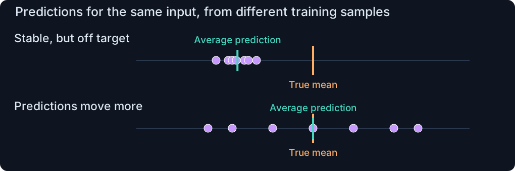
Repeated fitted predictions can have an off-target average or a wide spread

Bias: is the average on target?

Bias is the systematic error from a mismatch between the average learned relationship and the true one.
Example: a straight-line model misses a quadratic pattern.

Variance: how much do predictions move?

Variance is the variability of the learned model across possible training datasets from the same population.
Here, compare the spread of predictions at the same input.

Bias is the systematic difference between the average learned relationship and the true relationship. At a fixed input, compare the average fitted prediction across repeated training datasets with the true mean response. For example, a straight-line model cannot capture a genuinely quadratic mean over the input range, so its average fit can miss that pattern.

Variance describes how much the learned model changes across possible training datasets sampled from the same population, while keeping the fitting procedure and sample size fixed. At one input, this is the spread of predictions across those fitted models. It describes variation across repeated training, rather than the noise of one fresh observation. A model can have low variance and still be consistently off target.

The orange mark is the true mean, the teal mark is the average fitted prediction and the purple dots are individual fitted predictions. In real data we do not know the true mean; a simulation makes this comparison visible.

01 · Bias–variance trade-off

Bias measures the average miss; variance measures instability

Keep input $x$ fixed and repeat training on possible datasets $𝒟$ from the same population.

Bias: the average prediction’s miss

Bias (f (x; 𝒟)) = 𝔼_{𝒟} [f (x; 𝒟)] - 𝔼_{ε} [y]

Average learned prediction minus the true mean.

Variance: changes across training samples

Var (f (x; 𝒟)) = {Var}_{𝒟} [f (x; 𝒟)]

Spread of learned predictions at the same input.

𝒟

= one possible training dataset

f (x; 𝒟)

= prediction after training on

𝒟

x

= the same input in every comparison.

𝔼_{𝒟}

= average across training datasets

{Var}_{𝒟}

= variance across those datasets

𝔼_{ε} [y]

= true mean response at

x

y

= a new, unseen response,

ε

= its random error.

New observation: $y$ is an outcome not used for training. Its $ε$ is the random difference from the true mean at $x$ . For example, another crop trial with the same fertilizer dose can give a different yield. “Fresh” simply means new: this observation was not used for training. The noise $ε$ is the observation’s deviation from the true mean, whereas a residual compares an observed value with a fitted model prediction.

Keep $x$ fixed and imagine training the same procedure on possible datasets $𝒟$ from the same population. The notation $f (x; 𝒟)$ explicitly means the prediction at $x$ after training on $𝒟$ . The semicolon separates the prediction input from the dataset used for learning.

$𝔼_{𝒟}$ averages over those possible training datasets. The true mean response at this fixed input is $𝔼_{ε} [y]$ : average the new, unseen response $y$ over its random error $ε$ . Bias is the average learned prediction minus that true mean. It can be positive or negative; the error decomposition uses its square.

Prediction variance measures how fitted predictions spread around their own average across training datasets. Its full expectation form is:

Var (f (x; 𝒟)) = 𝔼_{𝒟} [{(f (x; 𝒟) - 𝔼_{𝒟} [f (x; 𝒟)])}^{2}]

A less flexible family can miss part of the true relationship while moving less across samples. A more flexible family can capture the relationship better while following sample-specific noise. These are tendencies, not a guarantee for every dataset. Bias here is unrelated to the intercept sometimes being called a bias term.

01 · Bias–variance trade-off

Expected MSE = squared bias + variance + noise

At the same input $x$ , imagine training again and predicting a new observation $y$ . Average the squared prediction errors over these repetitions.

𝔼_{𝒟, ε} [{(y - f (x; 𝒟))}^{2}] = {[Bias (f (x; 𝒟))]}^{2} + Var (f (x; 𝒟)) + Var (ε)

The sum on the right is the expected Mean Squared Error (MSE).
MSE is RMSE without the square root: $RMSE = \sqrt{MSE}$ .

Model-dependent part

Squared bias: how far the average prediction misses.
Variance: how much predictions change across training datasets.

Irreducible noise for these inputs

$ε$ is the new observation’s random difference from its true mean.
This variation remains even if we predict that mean perfectly.

x

= fixed input,

y

= new, unseen response

𝒟

= training dataset

f (x; 𝒟)

= prediction learned from that dataset.

𝔼_{𝒟, ε}

= average over datasets and new observation noise

ε

= new observation noise, independent of

𝒟

𝔼_{ε} [ε] = 0

means zero mean error.

The simulation knows the true curve. With real data, compare validation error because the true bias and variance are usually unknown.

At a fixed input $x$ , consider a new observation $y$ and the prediction $f (x; 𝒟)$ learned from a random training dataset $𝒟$ . The expectation $𝔼_{𝒟, ε}$ averages over both repeated training and noise in a new observation. This is expected mean squared error (MSE), rather than the error of just one observed case.

New observation: $y$ is an outcome not used for training. Its $ε$ is the random difference from the true mean at $x$ . For example, another crop trial with the same fertilizer dose can give a different yield. This random error belongs to the new observation and is independent of the dataset used for training. It is not a training residual. Both sides of the displayed identity give the expected MSE: the right-hand side splits it into three contributions. MSE is the quantity inside the RMSE square root. Here the expectation is at one fixed input, rather than an empirical average over a finite test set.

The expected squared prediction error decomposes into the squared bias ${[Bias (f (x; 𝒟))]}^{2}$ , prediction variance $Var (f (x; 𝒟))$ and noise variance $Var (ε)$ . The new observation’s random error $ε$ is independent of the training dataset, has mean $𝔼_{ε} [ε] = 0$ and finite variance. Bias compares the average prediction with $𝔼_{ε} [y]$ , the true mean response.

The simulation uses noise standard deviation 0.3, so $Var (ε) = 0.09$ . Its known generating curve makes bias and variance measurable across repeated fits. They cannot generally be recovered exactly from one real dataset. MSE has squared response units; taking its square root gives RMSE.

Irreducible noise is relative to the information in the selected inputs. More relevant measured predictors can change that information. Use training data for fitting, validation for model choices, and the final test set for assessment.

01 · Bias–variance trade-off

See bias and variance at the same input

Compare degrees 0, 2 and 9. Purple dots show 60 fitted predictions. The blue dotted line marks the selected input x.

The simulation knows the true curve. With real data, compare validation error because the true bias and variance are usually unknown.

The simulation knows the true mean curve $𝔼_{ε} [y] = 2 + 1.2 x - 0.9 x^{2}$ . It adds independent normal noise with standard deviation 0.3. It fits the chosen degree to 60 independently noisy training samples, each with the selected number of cases. The sample-set control selects a reproducible group of samples.

Each fitted curve represents $f (x; 𝒟)$ for one training dataset. The chart draws 15 of these curves, their 60-model average and the true mean curve. At the selected input, all 60 predictions appear as purple dots. The average miss gives bias, and the spread gives prediction variance. The scores are squared bias, prediction variance, noise variance 0.09 and their sum: an approximation to expected test MSE at that input.

Try a constant model, the correctly shaped quadratic, and a flexible degree-9 model. Then change training sample size. The exercise concerns repeated training, not changing the test outcome or knowing the true function in a real application.

The blue dotted line is only a guide to the selected input. The purple dots are the predictions from the 60 fitted models. The simulation knows the true curve. With real data, compare validation error because the true bias and variance are usually unknown.

01 · Bias–variance trade-off

Fit on training data → choose on validation → assess on test

Each dataset has a different job. Example scores below are illustrative: lower RMSE is better.

1 · TRAINING SET

Fit the candidates

━ Degree 2━ Degree 9

Learn the coefficients of both curves from the same training cases.

2 · VALIDATION SET

Choose the degree

Predict different, held-out cases.
Lower validation error → choose degree 2.

3 · TEST SET

Assess the chosen model

Degree 2 selectedTest RMSE: 0.35One final assessment

Predict a third, untouched set.
Report how well the chosen model generalizes.

Choose before testing. If a test score makes you change the model, that set is now guiding selection.

The diagram uses three disjoint subsets. The training set supplies the observations used to estimate coefficients. Both candidate degrees are fitted using those training cases. The validation set contains different observations: compare the candidates’ predictions with those targets. In this illustrative example, degree 2 has validation RMSE 0.32, lower than degree 9’s 0.58, so we select degree 2. These numbers illustrate the decision and are not measurements from the interactive simulation.

Only after fixing the procedure do we use the untouched test set. Its illustrative RMSE of 0.35 estimates the chosen model’s performance on new cases. Validation and test RMSE need not match because they use different observations. The test score does not choose the degree. Refitting the selected procedure using training and validation data before final testing is also possible, provided all choices are already fixed.

Fit each candidate on training observations and compare validation error or cross-validation estimates. Choose the complete procedure, including degree and learned transformations, before using the final test set. Keep preprocessing within the training portion of each split.

Validation supplies evidence for choices; testing supplies a final assessment of those choices. If test results guide another choice, they no longer provide an untouched final assessment. Model complexity, uncertainty of estimates and prediction error answer related but distinct questions.

02 · Accuracy of estimates

A nonzero fitted slope can still reflect sampling noise

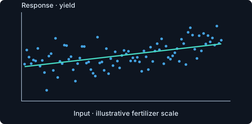
The 90 observations and their OLS fitted line

One sample gives one estimate

The fitted slope here is about 0.108. Another sample could give a different value.

The question: would a slope this far from zero be unusual* if the true population slope were zero?

A fitted number alone does not tell us how precise it is. We need its sampling uncertainty.

*Here, “unusual” means “unlikely to arise from sampling noise if the true population slope were zero.”

02 · Accuracy of estimates

A slope test asks about linear association

A fitted slope can be nonzero just because the sample is noisy. We state two hypotheses to check whether the data provide evidence of a linear association beyond this sampling variation.

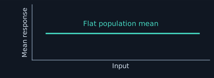
Null hypothesis

H_{0} : β_{1} = 0

The population slope is zero. A nonzero fitted slope can arise from sampling noise.

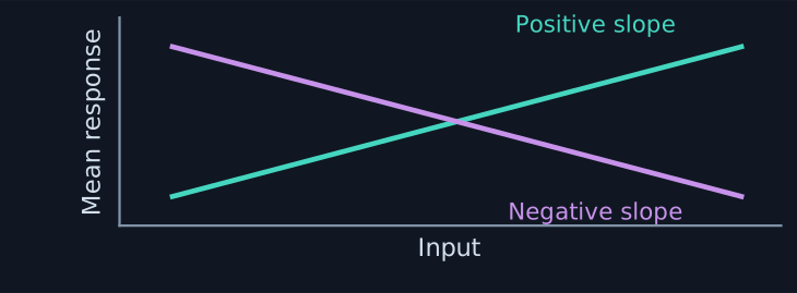
Two-sided alternative

H_{1} : β_{1} \neq 0

The population slope is positive or negative. The data may support a linear association.

Rejecting H₀ does not establish causation. Failing to reject does not establish no relationship.

β_{1}

= unknown population slope

{\hat{β}}_{1}

= its sample estimate.H₀ = zero-slope null hypothesis
H₁ = two-sided alternative.

A fitted slope can be nonzero just because the sample is noisy. We state two hypotheses to check whether the data provide evidence of a linear association beyond this sampling variation. Before looking at a p-value, we specify the claim to test and the competing possibility. This makes the evidence question precise: how unusual would the observed estimate be under the zero-slope hypothesis? The test does not decide that either hypothesis is certainly true.

The null hypothesis H₀: $β_{1}$ = 0 says that the population linear mean has zero slope. The two-sided alternative H₁: $β_{1}$ ≠ 0 allows either a positive or negative slope. A fitted slope will rarely be exactly zero even if the null is true, because estimates vary across samples.

Compare the estimate with its sampling uncertainty instead of comparing it with zero alone. Rejecting this null supplies evidence of a linear association under the assumptions. It does not establish causality. Failure to reject does not prove no relationship, especially if precision is low or the true relationship is nonlinear.

The small plots show illustrative population mean functions, not fitted samples. Under the null, the mean is flat even though individual observations may still be noisy. Under the two-sided alternative, the slope may be positive or negative: the two colored lines show separate possibilities, not two simultaneous fitted lines.

02 · Accuracy of estimates

Two different spreads: response scatter and slope uncertainty

RSE · Residual Standard Error

How scattered are the responses?

One fitted line, blue observed responses, and purple vertical residual gaps

Use one dataset. RSE estimates the size of the random scatter around its fitted line.

Units: response units, such as kg.

Slope SE · Standard Error of the Slope

How much does the fitted slope change?

Three lines fitted to different datasets, followed by a numbered axis with 20 slope estimates. Matching colors link the three lines to their slope estimates.

Repeat training on new datasets. Slope SE describes how much the slope estimates vary.

Units: response units per input unit.

The two panels answer different questions. The left panel uses one dataset and one fitted line. Each blue dot is an observed response. Each purple segment is a residual, the observed response minus the fitted prediction at the same input. RSE summarizes the estimated scatter around that line, in response units.

For the right panel, imagine repeating the study on new observations from the same population, while keeping the sample size, input values and fitting procedure fixed. Each dataset gives its own fitted intercept and slope. The upper plot shows three of these fitted lines. The matching colored dots on the lower numbered axis show their slope estimates. The other dots show the remaining estimates: one dot for each of 20 simulated datasets. Horizontal spread means the fitted slopes change across studies. The slope standard error describes the standard deviation of the slope estimate across such repetitions. In real data we estimate it from one sample using the formula introduced next. It has response units per input unit.

These teaching simulations use a mean response of 1 + 2x with independent normal errors. The left plot shows the first of the 20 simulated datasets. Each dataset contains 16 observations at the same inputs, with noise standard deviation 0.6. The lower axis uses all 20 slope estimates. The upper plot shows only three fitted lines to keep the comparison readable. A smaller slope SE means a more precise estimate. It does not by itself establish a large association or a causal effect.

02 · Accuracy of estimates

Repeated studies give different slopes: put them on one scale

This describes what fitted slopes would do across repeated studies. In ordinary data, the true $β_{1}$ and the true $σ$ are both unknown.

1 · Before: fitted slopes vary around the truth

{\hat{β}}_{1} \sim 𝒩 (β_{1}, σ^{2})

An illustrative distribution of fitted slopes centered at 2, with one standard error of 0.4.

Center = $β_{1}$ . Spread = $σ$ .

2 · Theoretical standardization

\frac{{\hat{β}}_{1} - β_{1}}{σ} \sim 𝒩 (0, 1)

The same distribution after subtracting its center and dividing by its standard deviation: mean zero and standard deviation one.

Center = 0, spread = 1.
Computing this needs the true $β_{1}$ and $σ$ .

β_{1}

= true population slope

{\hat{β}}_{1}

= slope fitted to one sample

σ

= true standard deviation of fitted slopes.

𝒩 (0, 1)

= normal distribution with mean 0 and standard deviation 1

\sim

means “has distribution”
Example: (2.4 − 2) / 0.4 = 1 standard error above the truth.

This theoretical quantity cannot be computed from the sample alone. A simulation can supply the true values. Next, estimate $σ$ from data.

The second block is a theoretical standardization, not an immediately computable sample statistic. Both the true population slope $β_{1}$ and the true sampling standard deviation $σ$ are unknown in ordinary observed data. The sample gives their estimates, not these population values themselves. The standardized expression can be evaluated only when the true values are supplied, for example by a simulation. It describes the sampling theory that motivates a practical test after a null slope is proposed and the standard error is estimated.

Imagine repeating the same simple-regression study while keeping its input values, sample size and fitting procedure fixed. The population slope $β_{1}$ is a fixed unknown number. Each new set of noisy responses gives a different fitted slope ${\hat{β}}_{1}$ . Under the classical normal-error assumptions, the distribution of these estimates is $𝒩 (β_{1}, σ^{2})$ . Here $σ$ denotes the true sampling standard deviation of the slope estimate, also called its true standard error.

Subtracting $β_{1}$ centers the distribution at zero. Dividing by $σ$ measures distance in standard-error units. A value of +1 means one standard error above the true slope, and −1 means one standard error below it. The plots use an illustrative true slope 2 and true standard error 0.4. A fitted slope 2.4 therefore becomes (2.4 − 2) / 0.4 = 1. These illustrative values are separate from the 90-observation example.

Distinguish the slope standard error $σ$ from the response-error standard deviation $σ_{ε}$ . Their exact relationship in simple regression is:

σ = \frac{σ_{ε}}{\sqrt{\sum_{i = 1}^{n} {(x_{i} - \bar{x})}^{2}}}

$n$ is the number of observations, $x_{i}$ is input i, and $\bar{x}$ is the input mean. Equivalently, the slope variance is the response-error variance divided by the centered input sum of squares. Exact under a correct linear mean, varying fixed inputs, and independent normal errors with common variance. The response errors have conditional mean zero, their variance is finite and common across cases, the inputs are not all equal, and inference requires n > 2. In practice $σ$ is unknown. We estimate it on the next slide.

02 · Accuracy of estimates

Estimate how much the fitted slope would change

We estimate the slope standard error with $\hat{σ}$ . Press Next: equivalent formulas appear from left to right, while the explanation follows the selected step.

1 · Start with RSE

\hat{σ} = \frac{RSE}{\sqrt{\sum_{i = 1}^{n} {(x_{i} - \bar{x})}^{2}}}

Think rise/run: RSE is vertical response noise. The denominator is horizontal input spread. Their ratio estimates slope uncertainty, not the slope itself.

2 · Substitute RSS

\hat{σ} = \sqrt{\frac{RSS}{(n - 2) \sum_{i = 1}^{n} {(x_{i} - \bar{x})}^{2}}}

Replace RSE² with RSS / (n − 2): two fitted coefficients use two degrees of freedom.

3 · Expand the residuals

\hat{σ} = \sqrt{\frac{\sum_{i = 1}^{n} {(y_{i} - {\hat{y}}_{i})}^{2}}{(n - 2) \sum_{i = 1}^{n} {(x_{i} - \bar{x})}^{2}}}

Expand RSS into squared residuals. This is the same formula, written using the individual observations.

\hat{σ}

SE ({\hat{β}}_{1})

: estimated spread across repeated studies.
A hat means estimated, not squared.
It is not the actual error

{\hat{β}}_{1} - β_{1}

of this one fit.
RSE = response scatter. RSS = sum of squared residuals.

n

= cases,

i

= case index.

x_{i}

= input,

\bar{x}

= input mean.

y_{i}

= response,

{\hat{y}}_{i}

= fitted response.
Smaller

\hat{σ}

means less sampling variability.

n - 2

residual degrees of freedom.

More response noise increases slope uncertainty. More cases or more input spread reduce it, all else equal. Requires n > 2 and varying inputs.

The true standard deviation of the fitted slope across repeated samples is $σ$ . We cannot observe it directly, so we calculate its estimate $\hat{σ}$ from one dataset. This is the same quantity often written $SE ({\hat{β}}_{1})$ . It describes uncertainty in the estimated slope, not the scatter of a single response.

The first formula has a rise-over-run intuition. RSE is vertical response noise, measured in response units. The square root of the centered input sum of squares measures horizontal input spread. Dividing converts the estimated vertical noise into uncertainty about the line’s slope, in response units per input unit. This is an intuition for the slope standard-error formula, rather than the ordinary rise-over-run calculation of the fitted slope.

The hat in $\hat{σ}$ means that the standard error is estimated. It is not $σ^{2}$ , and it is not the realized estimation error ${\hat{β}}_{1} - β_{1}$ of this particular fitted slope. It estimates the standard deviation of fitted slopes across hypothetical repetitions of the same model and sampling conditions. Smaller values mean less sampling variability in estimating the true population slope.

First estimate the response-error standard deviation $σ_{ε}$ with RSE. Then divide by the square root of the centered input sum of squares. If the observed inputs cover a wider range, the data provide more information about the tilt of a line.

Next substitute RSE² = RSS / (n − 2). The denominator n − 2 reflects that the intercept and slope were estimated from the same observations. Finally, expand RSS as the sum of squared residuals. The three displayed formulas are equal, rather than three alternative methods.

The sum over i runs over all n cases. For case i, $x_{i}$ is the observed input, $y_{i}$ the observed response, and ${\hat{y}}_{i}$ its fitted prediction. $\bar{x}$ is the mean input. Larger response noise increases the estimated slope uncertainty, while larger input spread or more observations can reduce it, all else equal. The residual degrees of freedom must be positive, n > 2, and the inputs must vary.

02 · Accuracy of estimates

A new example: height and weight

We record height and weight for 16 people. Can a line summarize how average weight changes with height?

Each dot is one person All 16 simulated height–weight observations, with height in centimetres and weight in kilograms. No fitted line is shown yet.

All 16 simulated height–weight observations, with height in centimetres and weight in kilograms. No fitted line is shown yet.

What have we measured?

Input: height, measured in centimetres.
Response: weight, measured in kilograms.

Four of the 16 observations:

Height (cm)	Weight (kg)
155	61.3
168	74.6
180	76.0
195	91.2

Illustrative simulated data. The plot shows all 16 observations. Table values are rounded.

First look at the observations. Next, fit a line and ask how much evidence its upward slope gives.

This introduces a new, illustrative height–weight dataset before discussing its fitted slope. There are 16 simulated adults, with irregular heights from 155 to 195 cm as the input and weights in kilograms as the response. The first sample's weights range from about 61 to 91 kg. Each plotted dot is one paired observation. All 16 pairs appear in the plot, while the table lists four rounded examples. These are teaching data rather than a real survey.

The observations are exactly those in the less-scattered sample of the later side-by-side comparison. OLS on the full, unrounded observations gives slope 0.60 kg per cm and estimated slope standard error 0.06 kg per cm. This introductory plot shows observations only. The following slide introduces the fitted slope, and the comparison then shows its fitted line alongside a second, more variable sample using exactly the same height values.

02 · Accuracy of estimates

Why test a slope before trusting the upward trend?

The line fitted to these height–weight observations slopes upward. Is this evidence of a population linear relationship, or could sampling noise produce it if the true line were flat?

For the sample just shown, the fitted slope is 0.6 kg per cm. This sample estimate is not automatically the population slope.

1 · Start with the proposed flat line

Temporarily assume $H_{0} : β_{1} = 0$ .
This is the zero-slope population model.

2 · Imagine repetitions under that model

Use the same sampling setup.
Noise can make a fitted sample line tilt upward or downward.

3 · Compare our result with that reference

Would a fitted slope as far from zero as ours be unusual?
If very unusual, it is evidence against the flat population line.

We assess the observed result assuming a zero slope. We do not calculate the probability that the true slope is zero. A linear association does not establish causation.

Go to the next slide for a visual intuition

The preceding slide introduced 16 simulated adult height–weight observations. Fitting a line to this sample gives slope 0.6 kg per cm. An extra centimetre of height is therefore associated with an extra 0.6 kg in the fitted mean weight, not an exact 0.6 kg difference between every pair of people. An upward sample line alone does not tell us whether the population slope is nonzero: sampling noise can produce a nonzero fitted slope even under a flat population mean.

The slope test temporarily assumes the zero-slope null $H_{0} : β_{1} = 0$ . We imagine repeating the study under that model and the same sampling setup, then ask how unusual a fitted result at least as far from zero as the observed one would be. If it would be very unusual under the zero-slope model, the data provide evidence against that model under the regression assumptions.

This is a conditional assessment of the observed result. It does not calculate the probability that the population slope is zero, and the hypothetical repetitions are a reference model rather than extra data we must collect. The next comparison holds the fitted slope, sample size and inputs fixed while changing residual noise, showing why uncertainty must enter the comparison. Evidence of a linear association does not establish causation.

02 · Accuracy of estimates

The slope test: assume → repeat → compare

Imagine the population line is flat. What slopes could noise alone produce in samples like ours?

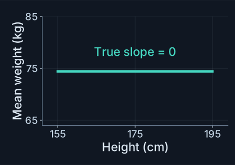
1 · Assume a flat population line Under the zero-slope assumption, population mean weight stays constant as height changes.

The true slope is temporarily set to zero. Individual responses can still be noisy.

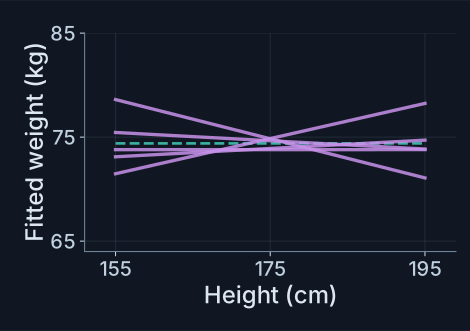
2 · Imagine repeated samples Five lines fitted to hypothetical samples generated around the same flat mean. Their estimated slopes tilt upward or downward because of noise.

Five lines fitted to hypothetical samples generated around the same flat mean. Their estimated slopes tilt upward or downward because of noise.

Keep the same 16 heights. Fit a new line to each hypothetical sample. Five of 500 fits are shown.

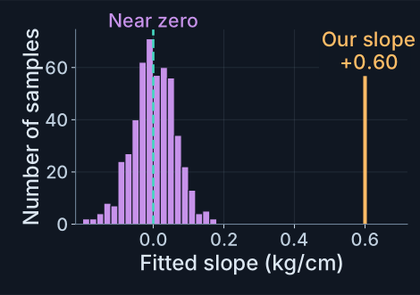
3 · Compare with our result A histogram of 500 fitted slopes from hypothetical flat-model samples is concentrated near zero. The observed slope plus 0.60 kg per cm is marked far to the right in orange.

A histogram of 500 fitted slopes from hypothetical flat-model samples is concentrated near zero. The observed slope plus 0.60 kg per cm is marked far to the right in orange.

Purple bars summarize all 500 fitted slopes. Our +0.60 kg/cm lies far from their cluster.

The t test asks whether our fitted slope could plausibly result from sampling noise when the true population slope is zero.

t < 0
Negative fitted slope.t = 0
Fitted slope equals zero.t > 0
Positive fitted slope.

For a positive estimated standard error. The sign shows direction, not strength of evidence.

This visual follows the same three steps as the preceding slide. First assume that mean weight does not vary with height: the population slope is zero. The horizontal teal line shows that assumed mean, not a claim that every person's weight is identical. The flat level is the mean response in the 16-observation example.

Second imagine new responses at the same 16 height values. For this illustration, generate 500 hypothetical samples by adding independent normal response noise to that flat mean. Its standard deviation is set to the RSE estimated from the less-scattered height–weight sample. Fit an intercept and slope separately to every generated sample. The middle panel shows five of those fitted lines, spanning negative, near-zero and positive estimates. The dashed teal line remains the same assumed population mean.

Third collect all 500 fitted slopes into a histogram. Each purple bar counts hypothetical samples in a slope interval, rather than people. The orange mark is the slope +0.60 kg/cm computed from our original, non-flat-looking sample. It is much farther from zero than the simulated reference cluster. The histogram includes both negative and positive fitted slopes because noise can tilt either way.

This is a visual, plug-in noise simulation to explain the testing logic. It does not calculate an exact p-value or the probability that the null hypothesis is true. A finite simulation with no result as extreme as the observed one does not mean the true tail probability is zero. The formal test introduced later uses a t statistic and Student's t reference, accounting for estimation of the noise scale. Exact inference requires the stated regression assumptions. The following comparison shows why the same observed slope can provide different evidence when its uncertainty changes.

02 · Accuracy of estimates

The same fitted slope can give very different evidence

Two simulated adult height–weight samples: the same 16 height values, the same axis scales, and the same positive fitted slope. Only residual scatter changes.

Less vertical scatter Simulated adult height–weight data with fitted slope 0.60 kg per cm and estimated slope standard error 0.06 kg per cm.

{\hat{β}}_{1} = 0.60 kg/cm, \hat{σ} = 0.06 kg/cm, t = 10

Less vertical noise gives a smaller slope SE. Dividing the same fitted slope by this smaller SE gives a larger positive t.

More vertical scatter Simulated adult height–weight data with fitted slope 0.60 kg per cm and estimated slope standard error 0.30 kg per cm.

{\hat{β}}_{1} = 0.60 kg/cm, \hat{σ} = 0.30 kg/cm, t = 2

More vertical noise gives a larger slope SE. Dividing the same fitted slope by this larger SE gives a smaller positive t.

Slope SE also depends on sample size and horizontal input spread. Both are held fixed here, so this comparison isolates residual scatter. The t value is unitless.

Both plots use the same 16 irregular adult height values, from 155 to 195 cm, and the same fitted slope of 0.60 kg per cm. They share the same fitted intercept, height coordinates, observation count and axis scales. The fitted line predicts 75 kg at 175 cm. Only the residual scatter differs. These are illustrative simulated observations, not a real survey.

The residuals are centered and orthogonal to centered height, so scaling them preserves the fitted slope and intercept. Their scales give slope standard errors 0.06 and 0.30 kg per cm. Recomputing OLS from the displayed coordinates gives t = 0.60 / 0.06 = 10 for the less-scattered sample and t = 0.60 / 0.30 = 2 for the more-scattered sample. The two panels illustrate separate samples at matching heights, not weight changes of the same people.

The estimated response scatter RSE is approximately 2.8206 kg in the first sample and 14.1032 kg in the second. Their weight ranges are about 61–91 kg and 55–108 kg. The larger residual scatter increases slope uncertainty. Dividing the same fitted slope by its larger estimated SE gives a smaller positive t. Slope and slope SE both have kg/cm units, which cancel in the t ratio.

Slope SE also depends on sample size and input spread, both deliberately held fixed here. The next slide gives the t-statistic formula. This comparison illustrates evidence against a zero slope under the regression assumptions, not causation.

02 · Accuracy of estimates

The t statistic measures how far the slope is from zero

The numerator asks: how far is our fitted slope from the zero slope proposed by $H_{0}$ ? Divide that signed distance by its estimated standard error.

t_{observed} = \frac{{\hat{β}}_{1} - 0}{\hat{σ}} = \frac{{\hat{β}}_{1}}{\hat{σ}}

{\hat{β}}_{1} - 0

= signed distance from the tested zero slope.
Positive above zero, negative below. Absolute value ignores direction.
The zero comes from

H_{0}

, not from an estimate of the true slope.

{\hat{β}}_{1}

= fitted slope,

\hat{σ}

= estimated slope SE.

t_{observed}

= value computed from our observed data.

The t value measures deviation from a hypothetical zero slope in estimated standard errors. It does not give the probability that the true slope is zero.

Zero is subtracted because it is the population slope proposed by the null hypothesis. We temporarily assume the true slope is zero and assess how unusual the observed fitted slope would be under that assumption, relative to its estimated standard error. The numerator ${\hat{β}}_{1} - 0$ is the signed distance between the slope fitted to our data and the zero slope being tested. It is positive above zero and negative below zero. Its absolute value gives distance regardless of direction.

The t value tells us how much the observed slope from our data deviates from a hypothetical zero slope, measured in estimated standard errors. The observed value $t_{observed}$ is fixed after fitting our dataset. Across hypothetical repetitions under the zero-slope null, the same calculation is random and is denoted $T$ . This test does not assign a probability to the true population slope being zero.

The null hypothesis is $H_{0}$ : $β_{1} = 0$ . Compare the fitted slope with that null value, then divide by its estimated standard error $\hat{σ}$ . The observed ratio $t$ counts how many estimated standard errors the slope is from zero. Its sign indicates the direction, while its absolute value measures distance.

If the null and the classical assumptions hold, the random ratio from repeating the entire study follows Student’s t distribution with n − 2 degrees of freedom. Before data are observed this is a random quantity. Once a dataset is fitted, t is one realized value. We use the distribution to judge that realized value. Student’s t is symmetric and centered at zero, with heavier tails than the normal distribution. Estimating the unknown spread introduces the extra uncertainty that this reference distribution accounts for.

For the 90 displayed observations, the slope is 0.1075379991 and its estimated standard error is 0.0179471258. Their ratio is 5.991934335, on 88 degrees of freedom. The number 5.99 is a distance in standard-error units, not a probability. A large absolute t is evidence to investigate against the zero-slope null, not proof of a causal effect. Exact under a correct linear mean, varying fixed inputs, and independent normal errors with common variance.

Use the controls to change the fitted slope or its estimated standard error independently. Hold the slope fixed and increase the standard error: the absolute t statistic becomes smaller. Near zero and Far from zero provide simple examples. The 90-point button restores the values calculated from the supplied data. These illustration controls change the displayed estimate and uncertainty directly. The data-generation example later shows how new observations produce such changes.

02 · Accuracy of estimates

A p-value compares our observed t with a zero-slope reference

Assuming the true line were flat, how rare would a t value at least as far from zero as ours be?

p-value = P (| T | \geq | t_{observed} | ∣ H_{0})

1 · One result from our observed data

t_{observed} = 2.2

Example: we compute this number once.
It is fixed by our original dataset.

2 · A random result in imagined studies

T

Assume $H_{0} : β_{1} = 0$ .
The same calculation on each hypothetical sample gives a new $T$ .
Same model and sampling setup, not extra data to collect.

3 · Count results at least as far from zero

T \leq −2.2 or T \geq 2.2

Absolute values ignore sign.
The inequality counts both directions, including equally extreme results.

If the observed t is zero

t_{observed} = 0 \Rightarrow p-value = 1

With a positive estimated SE, the fitted line is flat. Every possible $| T |$ is at least 0.
This gives no evidence against a zero slope, but does not prove it.

Choose the threshold before inspecting the result

$α$ = significance threshold (often 0.05, depending on the task).
$p-value < α$ : reject the zero-slope null.
$p-value \geq α$ : insufficient evidence to reject it.

Smaller p means stronger evidence against a flat population line. “More extreme” means farther from zero in t units, not a larger raw slope. It is not the probability that the null is true.

Assuming the true slope is zero, the p-value is the probability that a hypothetical repetition of the study gives a t value at least as far from zero as the t value we computed from our original data. These are hypothetical repetitions under the same model and sampling setup, not additional data we must collect. Compare absolute t values, rather than raw slopes.

The two quantities use the same t-statistic calculation but refer to different datasets. $T$ is a random statistic across hypothetical repeated samples under the zero-slope null. $t_{observed}$ is the fixed number already calculated from our actual dataset. The probability expression asks how often $| T |$ , a random distance, is at least $| t_{observed} |$ , our observed distance. The vertical bar means “assuming” or “given” $H_{0}$ .

Absolute value means distance from zero regardless of sign. In the illustrative case $t_{observed} = 2.2$ , the outcomes counted are $T \leq −2.2$ or $T \geq 2.2$ . An equally distant negative result is just as extreme as a positive one. “More extreme” does not mean a larger raw slope without regard to its standard error: it means a t statistic at least as far from zero.

A smaller p-value means that, if the true line were flat, a result like ours or more extreme would be rarer. Thus a small p-value is stronger evidence against a flat population line, under the regression assumptions. It does not give the probability that the population slope is zero, measure effect size, or establish causation. The p in p-value is unrelated to polynomial degree p.

If $t_{observed} = 0$ and the estimated slope standard error is positive, the fitted slope is zero and the fitted line is flat. Every possible absolute random t value is at least zero, so the two-sided p-value is 1. This gives no evidence against the zero-slope null; it does not prove the population slope is zero.

Choose a significance threshold $α$ before inspecting the result. The often-used value 0.05 is a convention whose appropriateness depends on the task and field. Reject the null when the p-value is below that threshold. Otherwise there is insufficient evidence to reject it, rather than proof of no relationship. A nonlinear relationship is not ruled out by failure to reject a zero linear slope.

The following interactive slide explores the same ideas. At observed t = 2.2 with 88 degrees of freedom, the two-sided p-value is approximately 0.0304. This is distinct from the supplied 90-observation fit, whose t is approximately 5.99193 and whose p-value is approximately 4.445 × 10⁻⁸. The null reference distribution and interpretation require the stated simple-regression assumptions: a correct linear mean, varying fixed inputs, and independent normal errors with common variance and mean zero.

02 · Accuracy of estimates

Explore the observed t and both probability tails

Change the observed t, n or threshold α. Try t = 0, switch its sign, or load the 90-point result. Watch the decision change as p crosses α.

The curve describes repeated studies under $H_{0}$ . A larger distance from zero leaves less probability in the two tails.

The curve is the Student t reference under the zero-slope population model. The control n is the number of observations in each hypothetical study. The calculation uses n − 2 degrees of freedom internally for a simple regression with an intercept and slope. Changing n updates the reference curve while holding the selected observed t fixed. It does not generate or refit a new dataset.

Start with t = 0: every absolute reference value is at least zero, so the two-sided p-value is 1. At observed t = 2.2 and n = 90 observations, the probability in both tails beyond −2.2 and +2.2 is approximately 0.0304. Reversing the sign of t leaves the two-sided p-value unchanged. Larger absolute t values leave less probability in the tails.

The decision compares the unrounded p-value with the selected significance threshold α. Show REJECT in red when p < α, meaning reject the zero-slope null. Show DON'T REJECT in yellow when p ≥ α, meaning there is insufficient evidence to reject that null. Equality belongs to DON'T REJECT. A failure to reject does not prove that the population slope is zero, and rejection does not establish causation. Changing α changes the decision threshold without changing the p-value.

The 90-point result button loads the fitted statistic from the supplied dataset and sets n to 90. Its observed t is approximately 5.99193 and its two-sided p-value approximately 4.445 × 10⁻⁸. This is a separate dataset from the 16-observation height–weight illustration. The default t = 2.2 is an independent illustration, not a fit to those 90 points.

The shaded probability includes tails beyond the plotted limits. Curve height is density, while shaded area represents probability. The reference and its interpretation require a correct linear mean, varying inputs, and independent normal errors with common variance and mean zero. These are hypothetical zero-slope repetitions, not additional data that must be collected.

02 · Accuracy of estimates

Follow one complete test: fit, estimate uncertainty, compare

Start with the supplied data. Then simulate new samples: change their size, noise, true slope or input spread. Compare the OLS line with a mean-only fit.

All quantities in this example are calculated from the same 90 plotted observations. First OLS fits an intercept and slope, choosing the coefficients that minimize RSS. The estimated slope is ${\hat{β}}_{1} \approx 0.107538$ . This is the estimated change in mean response per unit of input.

Second, calculate the response scatter RSE ≈ 0.0496994 and use the centered input spread to obtain $\hat{σ} \approx 0.0179471$ . RSE and the slope standard error have different roles and units. Third, test the zero-slope null by dividing the fitted slope by its estimated standard error: t ≈ 0.107538 / 0.0179471 ≈ 5.99193. The estimate is almost six standard errors above zero.

Fourth, use Student t with n − 2 = 90 − 2 = 88 degrees of freedom. The two-sided probability beyond ±5.99193 is about 4.445 × 10⁻⁸. At α = 0.05 this rejects the zero-slope null. The interpretation is evidence of a linear association under the assumptions, not proof of a practically large or causal effect.

Hiding the line only changes the picture, not the observations or calculated statistics. Zoom, pan and reset help inspect the scatter. The next question’s p-value of 0.03 describes a separate hypothetical study, while this fitted dataset has the much smaller p-value reported above. Exact under a correct linear mean, varying fixed inputs, and independent normal errors with common variance.

The data control begins with the supplied 90 observations and the same fitted statistics as the worked example. Choose Simulate new data or New simulated sample to explore a known linear population. The generator is $y_{i} = 0.5 + β_{1} x_{i} + ε_{i}$ , with independent normal errors of mean zero and the selected response-noise standard deviation. Inputs are evenly spaced around 0.5, over the selected narrow or wide range. A sample set selects a reproducible noise realization. The new-sample button changes that realization.

Vary one feature at a time: use fewer cases, increase noise, narrow the input spread, or set the true slope to zero. Each change refits OLS and recalculates the slope, its estimated standard error, t, the two-sided p-value, training RSE and RSS. Sampling variability means a nonzero population slope can fail to give a significant sample result, and a zero population slope can occasionally produce a false positive.

Compare OLS with the mean-only fit, which always predicts the observed response average and has zero fitted slope. Its RSS is TSS. Both fits use the same observations, and the displayed slope-test statistics continue to describe the OLS fit. The dashed generating mean is shown only for simulations, where that mean is known.

The interpretation now spells out the reason for the decision in three linked steps. First divide the estimated slope minus the tested zero by its estimated slope standard error to calculate t. Its absolute value is the distance from zero in estimated slope SEs. Next compare the two-sided p-value with α = 0.05. Show REJECT if p < α and DON'T REJECT if p ≥ α. Finally explain whether a t value this far from zero would be rare under a flat population mean. A failure to reject is insufficient evidence against zero, not proof that the slope is zero. The displayed formulas are rounded for reading, while decisions use the unrounded p-value. The calculation and explanation update together when data settings change.

02 · Accuracy of estimates

A confidence interval adds an uncertainty margin to the slope

Start with the worked 95% interval. Then repeat the study: each new dataset gives a new fitted slope and a new interval.

{\hat{β}}_{1} \pm t_{0.975, n - 2} \hat{σ}

{\hat{β}}_{1}

= fitted slope,

\hat{σ}

= estimated slope standard error
n = cases in each study. Every interval uses n − 2 degrees of freedom.
The t multiplier leaves 2.5% in each tail.About 95% of intervals from repeated studies cover the fixed true slope.
That long-run rate does not require exactly 19 hits in every group of 20.
The simulation knows the true slope, so it can show which intervals miss.

This is an interval for the population slope, not for an individual future response. It does not establish causation.

A fitted slope is a point estimate. A confidence interval adds a sampling-uncertainty margin around that estimate. For a two-sided 95% interval, multiply the estimated slope standard error $\hat{σ}$ by the Student t critical value $t_{0.975, n - 2}$ , then subtract and add the resulting margin to ${\hat{β}}_{1}$ .

The critical value is the 97.5th percentile: 97.5% of the reference probability is to its left and 2.5% to its right. Symmetry leaves another 2.5% below the negative critical value, so 95% lies between the two cutoffs. For n = 90 the degrees of freedom are 88 and the multiplier is about 1.987. Thus 0.107538 ± 1.987 × 0.0179471 gives approximately [0.0719, 0.1432].

The blue point is the fitted slope and the teal segment is the confidence interval. Zero lies outside it. Under the same assumptions, excluding zero agrees with rejecting the two-sided zero-slope test at α = 0.05. An interval that includes zero would not provide evidence to reject that null at this threshold.

The 95% refers to coverage across repeated studies: about 95% of intervals constructed by this procedure would contain the fixed true slope. It is not a 95% posterior probability that this already observed interval contains the slope, and it does not mean 95% of future responses fall in this interval. It concerns a population coefficient, not an individual future response. It also does not establish causality. Exact under a correct linear mean, varying fixed inputs, and independent normal errors with common variance.

The interactive example starts with the 95% interval calculated from the 90 supplied observations. Select 20 repeated studies, or press Repeat 20 studies, to generate 20 independent datasets with a known population slope of 0.10 and intercept 0.5. Each study uses the selected sample size and independent normal response errors with the selected standard deviation. Inputs are evenly spaced from 0 to 1. OLS and its standard error are recalculated separately for every dataset.

Each horizontal segment is one 95% confidence interval, with its fitted slope marked. The orange vertical line is the known true slope. Teal intervals cover that value and red intervals miss it. Use Inspect interval to see any row’s estimate, estimated standard error, t multiplier and endpoints. The selected fitted slope is marked in blue.

Increasing sample size or reducing response noise tends to narrow intervals. Repeat the group to see that the number covering the true slope varies. The 95% statement concerns the long-run coverage of the procedure, rather than an exact requirement that 19 out of each group of 20 intervals cover. All intervals retain the 95% level and use their own n − 2 degrees of freedom.

03 · Multiple linear regression

One response can depend on several useful predictors

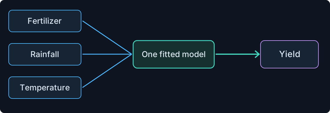
Fertilizer, rainfall and temperature enter one model predicting yield

Multiple linear regression combines several measured inputs in one prediction rule.

03 · Multiple linear regression

Several predictors, one response: fit their coefficients together

\begin{matrix} y_{i} = β_{0} + β_{1} x_{i 1} + \dots + β_{m} x_{i m} + ε_{i} \\ y_{i} = \sum_{j = 0}^{m} β_{j} x_{i j} + ε_{i} \end{matrix}

y = X β + ε

n = observations, i = case index
m = predictor count, j = predictor index
xᵢⱼ = input j for case i, with xᵢ₀ = 1.
yᵢ = observed response for case i.βⱼ = coefficient for input j,

β_{0}

= intercept
εᵢ = random error for observation i
X has n rows and m + 1 columns.

y and ε stack the n responses and errors. β stacks m + 1 coefficients. Each row of X is [1, xᵢ₁, …, xᵢₘ].

03 · Multiple linear regression

Change one input while keeping the others fixed

A multiple-regression coefficient describes a comparison at the same values of the other included predictors.

Predicted yield = 1 + 2 F + .5 R

Case A: F = 1, R = 4

Predicted yield = 1 + 2 × 1 + 0.5 × 4 = 5.

Case B: F = 2, R = 4

Predicted yield = 1 + 2 × 2 + 0.5 × 4 = 7.

F = fertilizer input, R = rainfall input
The example uses illustrative input and yield units.Rainfall stays at 4. Raising fertilizer by 1 raises the model prediction by 2.
That is the meaning of the coefficient 2.

This is a model-based conditional association. A causal effect needs additional evidence about the study and mechanism.

The coefficient βⱼ is the modeled change in mean response per unit of predictor xⱼ, holding the other included predictors fixed. The simple example uses predicted yield = 1 + 2F + 0.5R, where F is fertilizer and R is rainfall in illustrative units.

At F = 1 and R = 4 the model predicts 5. At F = 2 with the same R = 4 it predicts 7. The two-unit change for a one-unit increase in F is the fertilizer coefficient, 2. Holding the other inputs fixed defines the comparison; it does not by itself make it an experiment or a causal effect.

When included predictors are correlated, their individual coefficients can be unstable. Holding one input fixed while changing another may also describe combinations scarcely observed in the data, relying on extrapolation. Adding a variable changes the conditional question answered by a coefficient.

03 · Multiple linear regression

Ice-cream sales and shark attacks: the regression result

Imagine recording ice-cream sales and shark attacks at different times of year. These illustrative values are normalized to show the pattern.

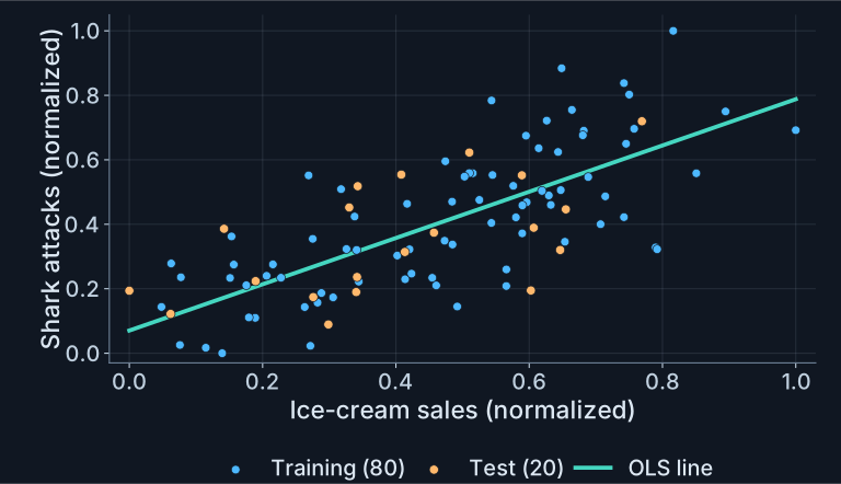
Predictor: sales → response: attacks The original 80 training and 20 test observations of normalized ice-cream sales and shark attacks, with the upward OLS fitted line.

The original 80 training and 20 test observations of normalized ice-cream sales and shark attacks, with the upward OLS fitted line.

A tempting causal claim

“More ice cream must be causing the attacks!”

The line rises, R² ≈ 0.53, and the slope test gives p < 0.01. These support a linear association.

What can we actually conclude?

Sales and attacks vary together.
The regression alone does not explain why.

R²Coefficient of determination	RSEResidual standard error	Test RMSERoot mean squared error	Slope tTest statistic	Slope p-valueTwo-sided test
0.5300	0.1525	0.1487	9.3792	< 0.01

Consider the familiar ice-cream and shark-attack example. Imagine recording sales as a predictor and attacks as an outcome across different times of year, then fitting a simple linear regression. The plotted values are illustrative normalized indices rather than a documented real-world survey or a causal experiment. The chart contains 80 training observations and 20 test observations, the same points used in the later interactive example.

The upward fitted line gives evidence of a positive association between the two indices. Recomputing OLS from the 80 training observations gives intercept 0.0703611652 and slope 0.7176136662. The training R² is 0.5300353268, training RSE is 0.1524972516, and RMSE on the separate 20 test points is 0.1487342609. R² compares the model with the mean-only baseline, RSE estimates residual scatter on training data, and test RMSE measures predictive error on the held-out cases. Error values use the normalized response scale.

The slope t statistic is 9.3792282024 on 78 degrees of freedom, with two-sided p-value approximately 1.987 × 10⁻¹⁴. The table reports p < 0.01 for readability. These results concern a nonzero population linear slope under the regression assumptions. The fitted model line matches OLS on the shown training points.

A tempting but unjustified leap is to conclude that eating or selling more ice cream causes more shark attacks. A positive slope, a moderate R² and a small association p-value cannot establish that intervention claim. The data show that sales and attacks vary together, without identifying the mechanism. A common cause could affect both. The next slide states the correlation-versus-causation principle with a humorous illustration, and the following slides investigate the shared-temperature explanation.

03 · Multiple linear regression

Correlation does not imply causation

In our example, ice-cream sales and shark attacks rise together. Should we arrest the ice-cream vendor?

The absurd conclusion On a sunny beach, a two-scoop ice cream in a waffle cone says I plead delicious. A clearly drawn shark with a dorsal fin, gills and forked tail replies Don’t blame the sprinkles.

On a sunny beach, a two-scoop ice cream in a waffle cone says I plead delicious. A clearly drawn shark with a dorsal fin, gills and forked tail replies Don’t blame the sprinkles.

A possible common cause: hot weather

Warm days can increase both ice-cream sales and swimming. More swimmers means more exposure to sharks.

The association alone does not show that ice cream causes shark attacks.

Correlation: two quantities vary together.
Causation: changing one produces a change in the other. A correlation alone cannot establish that.

More examples: Tyler Vigen’s Spurious Correlations ↗

The joke is to treat the ice-cream vendor as the culprit because ice-cream sales and shark attacks rise together in the teaching example. The cone protests “I plead delicious”, and the shark replies “Don’t blame the sprinkles”. This deliberately absurd conclusion illustrates that an association, even one with a small regression p-value, does not by itself establish a cause.

Hot weather is a plausible common cause to investigate. Warmer conditions can increase demand for ice cream and encourage more swimming. More people in the water can increase exposure to sharks and contribute to the observed attack pattern. This is a proposed mechanism, not something established by the sales–attack scatterplot. The chart in the next slide uses illustrative indices and is not a causal experiment.

Correlation describes how two quantities vary together. Causation asks whether deliberately changing one would change the other. A sales–attack association alone therefore cannot tell us whether reducing ice-cream sales would reduce shark attacks. Common causes, study design and assumptions about the mechanism matter. Correlation may be compatible with causation, but it cannot establish it on its own. The next slides inspect the association and develop the common-temperature explanation, followed by a controlled adjustment example.

03 · Multiple linear regression

Association alone cannot identify the cause

These illustrative sales and attack indices rise together. Inspect the points: can this two-variable scatter tell us whether a third variable drives both?

03 · Multiple linear regression

A common cause can create an association

A confounder is a shared cause that can create or distort the association between a predictor and an outcome.

Higher temperature may affect both ice-cream sales and exposure to swimming. This is a causal hypothesis to investigate.

A confounder is a shared cause of the predictor and the response. The arrows below propose temperature as one possible explanation of the association. A diagram states a mechanism to investigate; a scatterplot alone does not establish those arrows.

A confounder is a common cause of a predictor and an outcome that can create or distort their association. The proposed diagram gives temperature arrows toward both ice-cream sales and shark attacks, with swimming exposure providing a plausible link to attacks.

A causal diagram records assumptions about a mechanism; it is not inferred from the two-variable scatterplot. Assessing the mechanism needs appropriate observations and study design. A statistically significant simple slope cannot distinguish a direct effect from this shared-cause explanation.

03 · Multiple linear regression

Adjustment compares cases at the same temperature

SharkAtt = β_{0} + β_{1} IceCreamSales + β_{2} Temp + ε

Without temperature

The ice-cream sales coefficient is the slope multiplying the sales input. It can also capture the shared warm-weather pattern.

With temperature

$β_{1}$ : predicted shark-risk change for +1 sales index, at fixed temperature.
$β_{2}$ : predicted change for +1 temperature index, at fixed sales.

SharkAtt = shark-attack outcome
IceCreamSales = sales predictor.
ε = random response error.Temp = temperature predictor

β_{0}

= intercept

β_{1}

= ice-cream sales coefficient

β_{2}

= temperature coefficient

Adding temperature changes the comparison: sales is now compared at the same temperature. The coefficient and its uncertainty can both change.

The model includes ice-cream sales and temperature as separate predictors of the shark-attack outcome. $β_{1}$ now describes the association with sales while holding temperature fixed; $β_{2}$ describes the association with temperature while holding sales fixed. This is a different comparison from a regression using sales alone.

A coefficient that becomes smaller or less statistically precise after adjustment is compatible with a shared-temperature explanation. This is a possible mechanism to investigate, not a claim established by the displayed scatterplot. Temperature observations are needed to estimate this adjusted model; the available sales–attack chart alone is insufficient. Appropriate study design remains necessary for causal conclusions.

A coefficient is the number multiplying a predictor in the model. “Sales coefficient” and “ice-cream coefficient” both mean the coefficient of ice-cream sales, not sales themselves or a correlation score. With temperature included, $β_{1}$ describes the modeled response change for one extra sales-index unit while temperature stays fixed, and $β_{2}$ describes the change for one extra temperature-index unit while sales stay fixed. The fitted model estimates these coefficients from the sample.

03 · Multiple linear regression

Try the same data with and without temperature

Choose the model. In Sales + temperature, select sales or temperature on X. Shark risk stays on Y.

This controlled simulation generates 80 observations. Temperature varies, the sales index responds to temperature plus independent noise, and the attack-risk index responds to temperature plus independent noise. Sales has no direct term in the outcome generator. These are teaching indices rather than observed counts or evidence about real shark attacks.

In the sales-only view, the fitted slope mixes the common temperature pattern into the sales association. Include temperature to fit an intercept and both predictor coefficients jointly. The displayed line then compares predictions at the sample’s mean temperature, making the conditional meaning concrete. Points keep their temperature colors and the data stay unchanged when the model changes.

Sample set A gives a strong positive sales-only slope. After adjustment, the sales coefficient is close to zero and its p-value is much larger, while the temperature coefficient remains clear. The p-values are calculated from each model using the appropriate coefficient standard errors: 78 residual degrees of freedom for the simple line and 77 for the intercept plus two predictors.

Sample set B deliberately remains available even though random noise gives a small adjusted sales p-value in that sample. The generator still has no sales term. A significance decision can be a false positive; it is not a guarantee or a proof of mechanism. Sample set C gives another reproducible sample.

The labels now consistently say ice-cream sales coefficient and temperature coefficient. The ice-cream sales coefficient is also sometimes shortened to sales coefficient or ice-cream coefficient: all three names refer to the same model multiplier. A coefficient is a predicted change in shark-risk index per extra unit of its input index. In the model including temperature, the other input is held fixed. In the sales-only model there is no temperature term, so its coefficient is not estimated or shown. The live explanation translates each fitted value into a predicted increase or decrease.

The X-axis choices now match the selected model. Sales only fixes X to ice-cream sales, because that is its sole predictor. Sales + temperature lets X show ice-cream sales or temperature. Shark risk remains fixed on Y in every view. Switching from an adjusted temperature view to Sales only automatically returns X to sales. Predictor–predictor and reversed-axis selections are not offered.

The same 80 observations and fitted coefficients remain unchanged when X changes. The plotted model slice varies the selected predictor while holding the other included predictor at its sample mean. With X set to sales, the adjusted line holds temperature fixed. With X set to temperature, it holds sales fixed. Dot color represents the other predictor. These views all match the model outcome, shark risk.

04 · Assumptions

LINE (1/2): the mean and independent errors

LINE is a memory aid for four assumptions of classical linear regression:
Linearity, Independence, Normality and Equal variance.
They help justify the standard errors and p-values used to judge uncertainty in fitted coefficients.

L · Linearity

The average response follows a weighted sum of the chosen features.

Intuition: A line describes the middle of the data. Individual observations can sit above or below it.

Why it matters: A missed curve can produce systematically wrong predictions.

I · Independence

The errors of different observations are independent.

Intuition: An error in one case gives no clue about the next. Repeated measurements of one person may break this.

Why it matters: Related errors can make standard errors and p-values misleading.

ε_{i}

= unobserved error for case i

X

= observed feature matrix

E [ε_{i} | X] = 0

: errors average to zero at each input
E denotes the mean over possible errors

Linearity is in the coefficients. Using x² as a feature can still describe a curved mean (x = input).

LINE is a memory aid for four assumptions of classical linear regression: L stands for Linearity, I for Independence, N for Normality, and E for Equal variance. These assumptions describe the modeled mean and the errors. They matter because classical standard errors and p-values rely on them to describe uncertainty in fitted coefficients. If the assumptions fail, the usual uncertainty calculations can be misleading. A small p-value or high R² cannot establish these assumptions.

Write the response as the modeled mean plus an unobserved error. $ε_{i}$ is the true response minus the population mean specified by the model, for observation i. It differs from the residual, which subtracts the fitted sample prediction. $X$ denotes the observed feature matrix, with one row per observation. Conditional notation means that we fix those feature values when describing the errors.

L means that the conditional mean is a weighted sum of the selected features, with coefficients entering linearly. A polynomial uses powers of the input as features and can still satisfy this requirement. The zero conditional error mean is $E [ε_{i} | X] = 0$ . If the chosen features omit a real curve, averaging more observations does not remove that systematic mismatch.

I means independence of the underlying errors across observations, conditional on the predictors. Repeated measurements on the same person, time series or shared group effects can create dependence. Treating such related cases as independent can misstate uncertainty. Independence does not require the predictor values to be evenly spaced.

A separate identifiability requirement for unique coefficients is full column rank: no feature column can be written as a combination of the other feature columns. For example, including both height in centimeters and exactly the same height in meters makes those columns redundant. Least-squares solutions can still exist when this condition fails, but individual coefficient values need not be unique.

04 · Assumptions

LINE (2/2): the shape and spread of errors

N describes the shape of the errors. E describes their spread. Both refer to errors at fixed input values.

N · Normality

At each input, errors follow a normal, bell-shaped distribution centered at zero.

Intuition: Small positive and negative errors are common. Large errors in either direction are rare.

Why it matters: Together with the other assumptions, this supports exact small-sample t tests.

E · Equal variance

Errors have the same spread at every input value.

Intuition: Predicting a larger response should not automatically mean a wider cloud of errors.

Why it matters: Unequal spread can make the usual standard errors unreliable.

Var (ε_{i} | X) = σ_{ε}^{2}

σ_{ε}^{2}

= common error variance
Var = variance, a measure of spreadEqual variance: homoscedasticity
Unequal variance: heteroscedasticity
“Given X” means fixing the observed input values

OLS can fit coefficients without normal errors. LINE supports classical inference about their uncertainty.

N and E describe the distribution of the unobserved errors after accounting for the mean response. Normality is a conditional assumption at each fixed input. It does not require the predictor values or the raw responses across all inputs to form a bell curve. N describes distribution shape, while E describes whether its spread changes across inputs.

Normality means errors at each input have a normal distribution centered at zero. Under a correctly specified mean, independent normal errors, equal variance and a full-rank design, the usual finite-sample t tests and confidence intervals are exact. OLS itself can minimize the sum of squared residuals without normal errors.

Equal variance means $Var (ε_{i} | X) = σ_{ε}^{2}$ for every case. $σ_{ε}^{2}$ denotes the common error variance, and Var is the variance operator. This condition is called homoscedasticity. Unequal variance is called heteroscedasticity. A fan-shaped residual cloud is one possible clue. With unequal variance, the usual homoscedastic standard-error formula may misstate uncertainty even if the mean model is appropriate.

The four illustrations are schematics, not data from a particular study. True errors are unobserved, so we use fitted residuals as diagnostic clues. Residual plots can reveal curvature, changing spread or patterns over observation order. A normal Q–Q plot checks distribution shape. Fitted residuals are generally dependent because of fitting constraints, even if the underlying errors are independent. A featureless plot does not prove all assumptions.

04 · Assumptions

Residual plots suggest the next question

Pattern	Possible concern	Next step
Curved mean pattern	Misspecified conditional mean	Consider justified features or transformations
Widening spread	Unequal error variance	Inspect scale; use suitable variance modeling or inference
Pattern over time or order	Dependent errors	Account for the sampling or temporal structure
Unusual isolated points	Outlier or influential observation	Check data quality and sensitivity

A featureless plot does not prove every assumption. A normal Q–Q plot compares residual quantiles with normal-distribution quantiles to assess shape.

Use residual plots to choose a follow-up question. A curved mean pattern suggests checking the conditional mean and suitable transformations. A widening spread suggests investigating variance or scale. Ordered runs suggest temporal or sampling dependence. An isolated point warrants a data-quality and sensitivity check.

Normality needs a different diagnostic, such as a normal Q–Q plot, and visual patterns are evidence rather than automatic verdicts. Fitted residuals are not the independent errors in the model; the fitting constraints generally make residuals dependent. The goal is to investigate the underlying mean and error process.

A normal Q–Q plot compares residual quantiles with the quantiles of a normal distribution. Approximate alignment along a straight reference line supports a normal-shape approximation, while systematic deviations suggest a mismatch. Residual plots remain diagnostic clues rather than proofs.

04 · Assumptions

A defensible regression workflow

Question

Define the outcome, intended use and units.

Data

Split cases to match the intended use.

Fit

Estimate the coefficients on training data.

Check

Compare validation error and residual patterns.

Assess

Test the chosen procedure and state assumptions.

Prediction quality, coefficient significance and causal evidence answer different questions.

04 · Assumptions

Reason before calculating

For n training cases, how many coefficients does a degree-5 polynomial have, and what is its full-rank RSE denominator?
Can a correctly calculated model score have negative R² on unseen test observations?
If the feature matrix X has redundant columns, can an ordinary least-squares solution still exist?
Does a slope p-value below 0.05 establish that ice-cream sales cause shark attacks?

n = number of training observations
X = matrix of input features.OLS = ordinary least squares
RSE = residual standard error.

04 · Assumptions

Explain the distinctions

01 · Parameter count

Six coefficients, including the intercept.
RSE denominator: n − 6, if n > 6 and rank is full.

02 · Baseline

Yes. Its predictions can be worse than the mean-response baseline on that held-out dataset.

03 · Existence

Least squares still has solutions, but coefficients may tie. A pseudoinverse chooses the solution with the smallest coefficient-vector length.

04 · Causality

No. The test concerns association under assumptions. Confounding and study design remain relevant.

n = training count
degree 5 means

β_{0}

,…,

β_{5}

.RSS = model squared-error sum
TSS = mean-baseline squared-error sum.

04 · Assumptions

Fit carefully. Evaluate separately. Interpret precisely.

Least squares minimizes squared residuals.
Polynomial features remain linear in coefficients.
Flexibility can improve fit and amplify instability.
Use validation for choices and testing for assessment.
Inference needs assumptions; association is not causation.

Next lecture: classification changes the target and the loss.

Sources & further reading

Uncertainty, inference and interpretation

From fitted predictions to uncertainty and interpretation

Five metrics: what does each one tell me?

Train again on new data: does the prediction move?

Bias measures the average miss; variance measures instability

Expected MSE = squared bias + variance + noise

See bias and variance at the same input

Fit on training data → choose on validation → assess on test

Fit the candidates

Choose the degree

Assess the chosen model

A nonzero fitted slope can still reflect sampling noise

A slope test asks about linear association

Two different spreads: response scatter and slope uncertainty

How scattered are the responses?

How much does the fitted slope change?

Repeated studies give different slopes: put them on one scale

Estimate how much the fitted slope would change

A new example: height and weight

Why test a slope before trusting the upward trend?

The slope test: assume → repeat → compare

The same fitted slope can give very different evidence

The t statistic measures how far the slope is from zero

A p-value compares our observed t with a zero-slope reference

Explore the observed t and both probability tails

Follow one complete test: fit, estimate uncertainty, compare

A confidence interval adds an uncertainty margin to the slope

One response can depend on several useful predictors

Several predictors, one response: fit their coefficients together

Change one input while keeping the others fixed

Ice-cream sales and shark attacks: the regression result

Correlation does not imply causation

Association alone cannot identify the cause

A common cause can create an association

Adjustment compares cases at the same temperature

Try the same data with and without temperature

LINE (1/2): the mean and independent errors

LINE (2/2): the shape and spread of errors

Residual plots suggest the next question

A defensible regression workflow

Question

Data

Fit

Check

Assess

Reason before calculating

Explain the distinctions

Fit carefully. Evaluate separately. Interpret precisely.

Further reading and practice

Continue the course